#generative adversarial networks

Generative Opposing Networks with Python Crash Course
Producing Generating Opposing Networks for Your Venture in 7 Days.
Generative opposing networks or brief GANs are a profound learning technique to practice generative fashions.
GAN research and their software are just a few years previous, however the outcomes achieved have not been vital. As the sector is so younger, it can be challenging to understand how to start, what to concentrate on and how greatest to use the obtainable methods.
On this crash course you will discover how one can begin and belief to develop in-depth studying about Generative Adversarial Networks using Python inside seven days.
Observe: This can be a great and essential message.
Discover the brand new GAN e-book with 29 step-by-step tutorials and full source code to be developed with DCGAN, Conditional GAN, Pix2Pix, CycleGAN and others
How to Get Started with Generative Adversarial Networks (7-Day Mini Course)
Photograph: Matthias Ripp, Some
Who is this collision course?
Before we begin, ensure you are in the best place.
The record under incorporates some common steerage on who this course is designed for
Don’t panic when you don’t match these factors accurately;
You have got to know:
- You’ve got a great basis for primary Python, NumPy and Keras training.
You don’t have to be
- Pc Science Researcher!
This collision course takes you from a developer who knows somewhat machine learning for a developer who can import GAN
Word: This crash course assumes you’ve a working Python 2 or three SciPy setting with at the least NumPy, Pandas, scikit-learning and keras 2. In the event you need assist in your setting, you’ll be able to comply with the step-by-step instruction here:
Overview of the Crash Course
This fall course is divided into seven classes.
You possibly can complete one lesson a day (really helpful) or full all the lessons in in the future (hardcore).
Under are seven classes that begin and produce with Python with Generative Adversarial Networks:
- Lesson 01: What are Generative Reverse Networks? 19659018] Lesson 02: GAN Ideas, Tips and Cages
- Lesson 03: Discrimination and Generator Models
- Lesson 04: GAN Loss Action
- Lesson 05: GAN Training Algorithm
- Lesson 06: GAN Lessons 19659018 ] Lesson 07: Superior GANs
Each lesson can take you anyplace from 60 seconds to 30 minutes. Take your time and take classes at your personal pace. Ask questions and submit the leads to the feedback under.
Lessons can anticipate you to go away and learn how to do issues. I’ll offer you clues, however a few of the lessons in each lesson are forcing you to study the place to go to find help for deep learning and GAN (tip: I have all of the answers to this weblog, simply use
Send results to comments; Lord you!
Keep there;
Observe: This is just a collision course. You’ll get rather more detailed and detailed guides, see my ebook on “Generative Adversarial Networks in Python.”
Lesson 01: What are generic opposing networks
On this lesson you will see that out what the GANs are
Generative Adversarial Networks or brief GANs are an strategy to generative modeling utilizing deep studying methods similar to convolutional neural networks
GANs are a sensible approach to develop a generative mannequin by framing an issue with a controlled studying drawback with two sub models: a generator mannequin practice to create new examples, and a mannequin of discrimination that tries to categorize examples as either actual (domain identify) or counterfeit (generated)
- Generator. A mannequin used to create new credible examples of the issue area.
- discriminator. A mannequin used to classify examples as actual (domain identify) or counterfeit (generated).
Two fashions are educated in a single zero-sum recreation, the other until the discrimination model is cheated about half the time. The generator model produces reliable examples.
Generator
The generator model takes a hard and fast size random vector as an enter and generates the image within the area.
The vector is randomly drawn from the Gaussian distribution (referred to as
) After the train, the generator mannequin is stored and used to generate new samples.
A real example is the tutorial materials
The separator is a traditional (and nicely understood) score model
After the coaching process, the discrimination mannequin is rejected because we are interested within the generator.
GAN training
Two fashions, generator
A single coaching session first includes choosing a batch of actual pictures from the problem area. Creating hidden dots and feeding the generator mannequin to synthesize a collection of pictures
Discrimination is then up to date utilizing and imaginary photographs, minimizing the loss of binary entropy utilized in all binary score problems.
The generator is then updated utilizing a discriminatory model. Which means the generated pictures are introduced to the discriminator as if they are real (not created) and the error is applied again to the generator mannequin. In consequence, the generator mannequin is updated in the direction of producing pictures which are more probably to be confusing discrimination
This course of is then repeated for a specific amount of exercise dogments
Your process
Your activity in this lesson is to record three potential purposes for Generative Adversarial Networks. You might get concepts for reviewing current research.
Submit the comments in the comments under. I’d like to see what you see.
Within the next lesson you will discover ideas and tips for the profitable coaching of GAN fashions.
Lesson 02: GAN Ideas, Hints and Cages
In this lesson
Generative Adversarial Networks is challenging to practice.
It’s because the structure consists of each a generator and a discrimination mannequin that compete in a zero sum recreation. One model enhancements are due to a deterioration in the efficiency of one other model. The result’s a really unstable coaching course of that may typically lead to failure, reminiscent of a generator that produces the same image all the time or generates nonsense
There are a number of heuristic or greatest practices (referred to as “GAN hacks”) that can be utilized in GAN. fashions and coaching. [19659003] Perhaps probably the most necessary steps in designing and training a secure GAN model is the strategy referred to as Deep Convolutional GAN or DCGAN.
This structure incorporates the seven greatest practices to think about when implementing a GAN model:
- Steady pattern using robust convolutions (eg Don’t use hyperlink layers)
- Upsample using stringent convolutions (eg Use transposed convolution layer)
- Use LeakyReLU (eg Don’t use commonplace ReLU). 19659018] Use batch normalization (eg Standardizing layer outputs after activation)
- Use Gaussian weight initialization (e.g., Average 0.zero and stdev zero.02).
- Use Adam Stochastic Gradient Descent (e.g. Studying Velocity 0.0002) and beta1 from 0.5.
- to Scale Photographs [-1,1] (eg use tanh at generator output.
These heuristics are profitable professionals who tested and evaluated lots of or hundreds of mixtures of assembly features for a number of issues.
Your process
Your activity on this lesson is to record three other GAN ideas or hacks that can be used in the course of the exercise. I’d like to see what you see.
Within the subsequent lesson you’ll discover out how simple discriminatory models and generator fashions could be carried out.
Lesson 03: Discrimination and Generator Mannequin
On this lesson you will notice how
We assume that the pictures in our area are 28 × 28 pixels in measurement and shade, which signifies that they have three shade channels.
Discriminator Model
* Separation mannequin accepts an image of 28x28x3 pixels and must classify it as real (1) or pretend (zero) by means of the sigmoid activation perform. . Each convolution layer descends from the end result utilizing 2 x 2 steps, which is the most effective apply for GANs, as an alternative of the merge layer.
Additionally according to greatest apply, the convolution layers are adopted by LeakyReLU activation with zero.2 and batch normalization layer
…
# defines the discrimination mannequin
mannequin = Sequence ()
# pattern for 14×14
mannequin.add (Conv2D (64, (three,three), Strides = (2, 2), padding = & # 39; similar & # 39; input_shape = (28,28,three)))
mannequin.add (LeakyReLU (alpha = zero.2))
model.add (BatchNormalization ())
# sample for 7×7
model.add (Conv2D (64, (three,three), steps = (2, 2), padding = & # 39; similar & # 39;))
model.add (LeakyReLU (alpha = zero.2))
mannequin.add (BatchNormalization ())
# Categorize
mannequin.add (Flatten ())
mannequin.add (Dense (1, activation = & # 39; sigmoid & # 39;))
… # define the pattern of discrimination model = Sequence () # pulldown 14×14 model .add (Conv2D (64, (3,three), Strides = (2, 2), padding = & # 39; similar input_shape = (28,28,3))) model.add ( LeakyReLU (alpha = zero.2)) model.add (BatchNormalization ()) # underscore 7×7 mannequin.add (Conv2D (64, (3.three), Strides = (2, 2) , padding = & # 39; similar & # 39;)) model.add (LeakyReLU (alpha = zero.2)) model.add (BatchNormalization ()) # Rank mannequin. add (Flatten ()) model.add (Dense (1, activation = & # 39; sigmoid & # 39;)) |
Generator Mannequin
Generator model takes a 100-dimensional level in a hidden state as input and generates 28x28x3.
The latent area point is the Gaussian vector random numbers. This is projected utilizing a dense layer 64 based mostly on a small 7 × 7 picture.
The small photographs are then dipped twice utilizing two transposed convolution layers with 2 × 2 steps followed by LeakyReLU and BatchNormalization layers which are
Output is a three-channel picture with pixel values in the vary [-1,1] tanh activation via.
…
# Specify the generator mannequin
model = Sequence ()
# Base for 7×7 pictures
n_nodes = 64 * 7 * 7
model.add (dense (n_nodes, input_dim = 100))
mannequin.add (LeakyReLU (alpha = zero.2))
mannequin.add (BatchNormalization ())
model.add (Reformat ((7, 7, 64)))
# sample for 14×14
mannequin.add (Conv2DTranspose (64, (3.three), Strides = (2,2), padding = & # 39; similar & # 39;))
mannequin.add (LeakyReLU (alpha = 0.2))
mannequin.add (BatchNormalization ())
# sample for 28 x 28
mannequin.add (Conv2DTranspose (64, (three.three), Strides = (2,2), padding = & # 39; similar & # 39;))
model.add (LeakyReLU (alpha = 0.2))
model.add (BatchNormalization ())
mannequin.add (Conv2D (three, (3,3), activation = tanh & # 39 ;, padding = & # 39; similar & # 39;)
1 2 three [19659083] 8 9 10 11 12 13 . ] 15 16 17 18 [19659129] … # outline the generator model mannequin = Sequence () # base for 7×7 n_nodes = 64 * 7 * 7 model.add (density (n_nodes, input_dim = 100)) model.add (LeakyReLU (alpha = 0.2)) model.add (BatchNormalization ()) mannequin. add (Reshape ((7, 7, 64))) [19659092] # sample 14×14 mannequin.add (Conv2DTranspose (64, (3,3), Strides = (2,2), padding = & # 39 the identical & # 39;)) mannequin.add (LeakyReLU (alpha = 0.2)) mannequin.add (BatchNormalization ()) # instance to 28×28 mannequin.add (Conv2DTranspose ( 64, (3.3), Strides = (2.2), padding = & # 39; similar & # 39; ) model.add (LeakyReLU (alpha = 0.2)) mannequin.add (BatchNormalization ()) model.add (Conv2D (three, (3,3), activation = & # 39 ; tanh & # 39 ;, padding = & # 39; similar & # 39;)) |
Your mission
Your activity on this lesson is to implement each discriminatory fashions and to summarize their construction.
For bonus points, upgrade models help a picture measurement of 64 × 64 pixels
Submit your comments within the comments under. I’d like to see what you see.
In the next lesson, yow will discover out how GAN model training strategies may be decided
Lesson 04: GAN loss features
On this lesson
Discriminator Loss
The separation mannequin is optimized to maximize the chance of figuring out the actual image from the fabric and generating the generator counterfeit or artificial pictures.
This can be carried out as a binary classification drawback where discrimination creates a chance for a specific picture zero and 1 between counterfeits and real ones.
The model can then be educated immediately and in batches of counterfeit photographs instantly and minimizes the adverse log chance most frequently carried out as a binary cross-entropy loss
As the perfect apply, the mannequin might be optimized using the Stochastic gradient Adam version with low studying and conservative velocity
…
# assemble the template
model.compile (loss = & # 39; binary_crossentropy & # 39; optimizer = Adam (lr = 0.0002, beta_1 = zero.5))
… # translation mannequin to model.comp (loss = & # 39; binary_crossentropy & # 39 ;, Optimizer = Adam (lr = 0.0002, beta_1 = zero.5)) |
Generator loss
The generator just isn’t updated instantly and there is no loss for this mannequin
.
That is achieved by making a composite mannequin through which the generator offers an image that instantly feeds the discrimination for classification.
The composite model can then be educated by providing random points in a hidden area as an input and discriminating that the ensuing photographs are actually actual. In consequence, the generator weights are updated to produce pictures which are more probably to be categorized as actual.
It is crucial that discrimination just isn’t up to date throughout this process and marked as untrained. [19659003] The composite model uses the identical class of cross entropy loss as an unbiased discrimination model and the identical stochastic gradient fall Adam version for performing optimization.
# creates a mixture mannequin for training the generator
generator = …
discriminatory = …
…
# Make weight in a discriminatory place not trainable
d_model.trainable = False
# Connect them
mannequin = Sequence ()
# add generator
model.add (generator)
# More Discrimination
mannequin.add (separator)
# assemble the template
model.compile (loss = & # 39; binary_crossentropy & # 39 ;, optimizer = Adam (lr = 0.0002, beta_1 = zero.5))
# creates a mixture mannequin to practice the generator generator = … [19659083] … # make weights in discrimination not trainable d_model.trainable = False # join them mannequin = consecutive () # more generator ] mannequin .add (generator) # extra separator mannequin.add (discriminatory) # translation model model.comp (loss = & # 39; binary_crossentropy & # 39 ;, optimizer = Adam (lr = zero.0002, beta_1 = zero.5)) |
Your mission
Your process on this lesson is to research and summarize the three loss features that can be utilized to practice GAN models.
Report the comments within the feedback under. I’d like to see what you see.
In the next lesson you can find the educating algorithm used to update the weights of the GAN model
Lesson 05: GAN Training Algorithm
In this lesson, find the GAN Coaching Algorithm
Defining GAN models is a troublesome part. The GAN training algorithm is comparatively easy
One cycle of an algorithm first consists of choosing a batch of precise pictures and utilizing the current generator patterns to type a batch of faux pictures. You’ll be able to develop small features to perform these two features.
These actual and faux pictures are then used to replace the discrimination model instantly by way of the call to Train_on_batch () Keras.
The points of the hidden area can then be the generated-generator-displacement mannequin for input, and the “actual” (class = 1) labels could be offered to replace the load of the generator model.
The exercise course of is repeated hundreds of occasions.
The generator mannequin could be periodically stored and downloaded later to verify the standard of the verified pictures.
The example under illustrates the GAN coaching algorithm
…
# gan-training algorithm
discriminatory = …
generator = …
gan_model = …
n_batch = 16
latent_dim = 100
for i in the space (10000)
# You get randomly chosen “real” samples
X_real, y_real = select_real_samples (material, n_batch)
# produces “counterfeit” examples
X_fake, y_fake = create_fake_samples (generator, latentti_dimi, n_batch)
# Creates training for discrimination
X, y = vstack ((X_real, X_fake)), vstack ((y_real, y_fake))
# Improve your weight model
d_loss = discrimination.train_on_batch (X, y)
# Put together points in a hidden area as a generator enter
X_gan = create_latent_points (latent_dim, n_batch)
# Creates reverse labels for counterfeit samples
y_gan = ones ((n_batch, 1))
# Replace the generator with a discrimination error
g_loss = gan_model.train_on_batch (X_gan, y_gan)
1
2
5
6
7
eight
eight
12
13
14
15
16
17
18
19
20
19 ] 22 [19659129[]
# gan training algorithm
discrimination = …
generator = …
gan_model = …
n_batch = 16
latent_dim = 100
for i within the area (10000)
# get randomly selected “real” samples
X_real, y_real = select_real_samples (material, n_batch)
# create & # 39; pretend & # 39; examples
X_fake, y_fake = create_fake_samples (generator, latent_dim, n_batch)
# creates trainee discrimination
X, y = vstack ((X_real, X_fake)), vstack ((y_real, y_fake))
] # update the weights of the discrimination model
d_loss = discrimination.train_on_batch (X, y)
# prepares factors in hidden area as input to the generator
X_gan = create_latent_points (latent_dim, n_batch)
# creates translated labels for pretend samples
y_gan = ones ((n_batch, 1))
# replace generator discrimination error
g_loss = gan_model.train_on_batch (X_gan, y_gan)
Your mission
Your process in this lesson is to tie together the weather of this and former classes and practice GAN with a small collection of photographs, reminiscent of MNIST or CIFAR-10.
Submit the feedback within the feedback under. I’d like to see what you see.
Within the subsequent lesson, you’ll be able to find out how to use GAN to translate a picture.
Lesson 06: GAN Pictures for Translation
In this lesson you can find GAN IDs
The interpretation between image and picture is managed conversion of a specific source image into a target picture. One example is the conversion of black and white pictures into colour pictures.
Translating photographs and pictures is a challenging drawback and sometimes requires specialized templates and loss features for a specific translation process or database.
GANs could also be educated to translate pictures and pictures, and two examples are Pix2Pix and CycleGAN.
Pix2Pix
Pix2Pix GAN is a common strategy to translating photographs and pictures.
The model is a educated database of paired examples where each pair accommodates an example of the image before and after the specified translation.
The Pix2Pix model is predicated on a conditional generative reverse community by which the goal picture is created, depending on the particular enter image.
The discrimination mannequin is given an image and an actual or shaped paired image and should determine whether or not the paired picture is actual or pretend.
The generator mannequin is given as a picture with a given picture and creates a translated version of the image. The generator model is educated both to confuse the discrimination mannequin and to reduce the loss of the resulting image and the expected image.
The Pix2Pix system employs extra advanced deep convolutional neural community fashions. Particularly, the U-Internet mannequin is used for the generator mannequin, and PatchGAN is used within the discrimination model.
Generator loss consists of a mixture of each the other lack of a traditional GAN model and L1 loss
CycleGAN
The limitation of the Pix2Pix mannequin is that it requires a mixed instance database before and after the specified translation.
where we might not have examples of translation, comparable to translating Zebra pictures into horses. There are other imaging tasks where there are not any such paired examples, corresponding to translating landscapes into pictures.
CycleGAN is a know-how that features automated training of translation models between picture and picture with out odd examples. Templates have been educated in an uncontrolled manner using supply code and destination domain photographs that do not want to be linked in any means.
CycleGAN is an extension of the GAN architecture, which includes the simultaneous training of two turbines
One generator takes pictures from the first area as enter and output alerts to one other domain, and the second generator takes footage from another domain as enter and generates pictures from the primary area. The discriminator fashions are then used to decide how reliable the generated photographs are and replace the generator patterns accordingly. This is the concept the image produced by the first generator might be used as an input to the second generator and the output of the second generator should correspond to the unique image. The reverse can also be true: the output of the second generator could be input as input to the primary generator and the outcome corresponds to the enter of the second generator
Your activity
Your process in this lesson is to listing 5 examples of the interpretation of the image it’s your decision to research with GAN models. I’d like to see what you see.
In the subsequent lesson you will see that a few of the latest advances in GAN models
Lesson 07: Advanced GAN
In this lesson you’ll discover some more superior GAN that exhibits vital results
BigGAN
BigGAN is an strategy that brings together a bunch of the newest greatest practices in training GANs and growing batch measurement and variety of model parameters.
means that BigGAN is focusing on expanding GAN models. Consists of GAN models with:
- Add mannequin parameters (eg Many other function maps).
- Bigger batch sizes (e.g. Tons of or hundreds of pictures).
- Architectural Modifications (eg Self-Information Modules). ] The resulting BigGAN generator model is capable of producing high-quality 256 × 256 and 512 × 512 photographs in many various picture categories
Progressive Rising GAN
Progressive GAN is an extension of the GAN coaching course of that permits secure training of huge, high-quality picture generator fashions.
Meaning beginning with a really small picture and regularly including layers of blocks that improve the output measurement of the generator models and the enter of the discrimination system.
Probably the most spectacular achievement of a progressive GAN is the creation of huge 1024 × 1024 pixel photorealistic generated faces.
StyleGAN [19659046] Fashion Generative Adversarial Community, or StyleGAN, is an extension to GAN structure that means main modifications to the generator model.
Consists of using a mapping network to map the dots of latent areas to an intermediate area, using latent area to control the type at every level of the generator model and the source of the noise variation at every generator model level
The ensuing mannequin isn’t capable of producing spectacularly high-quality, high-quality photographs of the face, but in addition supplies management The fashion of the produced picture at totally different levels of detail by altering type vectors and noise.
For example, blocks of synthetic network layers at decrease resolutions for high-level types akin to pose and coiffure, blocks at larger resolutions control shade preparations and very superb details akin to freckles and hair strands placement.
Your process in this lesson is to listing three examples of how you need to use patterns that may produce giant photorealistic photographs. I’d like to see what you see.
This was the final lesson.
The End!
(See how far you’ve come)You probably did it.
Take a second and look again to see how far you’ve come.
Found:
- GANs are a deep learning method that can produce generative fashions that can synthesize top quality photographs.
- Training GANs are inherently unstable and vulnerable to failures that can be solved by adopting greatest practices in the design, meeting and training of GAN fashions
- Generator and discrimination models utilized in GAN architecture might be defined merely and instantly
- […]
- The generator mannequin has been educated by the discrimination mannequin in the architecture of the mixture mannequin.
- resembling a translation between an image and an image in pairs and an odd example.
- Progress of GANs, corresponding to scaling fashions and gradual progress of models, permits
Subsequent Step and Examine My Ebook on Generative Racing Networks with Python
Abstract
How did you do with the mini-course?
take pleasure in this crash course?Do you will have any questions? Had any attachment points?
Inform me. Depart a comment under.Develop Generative Aggressive Networks At the moment!
Develop your GAN mannequin in minutes
… just some strains of python code
Discover the brand new eBook:
Generative Adversarial Networks with PythonIt provides self-study and end tasks:
DCGAN, Conditional GANs, Picture Translation, Pix2Pix, CycleGAN
and far more …Lastly deliver GAN fashions to vision tasks
Skip academicians. Only outcomes.
Click on for extra info
The post How to Get Started with Generative Adversarial Networks (7-Day Mini Course) appeared first on Android Illustrated.
Wasserstein Generative Adversarial Network (Wasserstein GAN) is an extension to a generic opposing network that improves each stability when training a mannequin and dropping a perform that correlates with the quality of the created photographs.
WGAN has a dense mathematical motivation, although in follow only a few minor modifications to the established deep convolution-related generative reverse community, or DCGAN.
On this tutorial you will find out how Wasserstein’s generic anti-competitive network might be carried out from scratch
When this tutorial is completed, you realize:
- Variations between the usual deep convolutional channel and the brand new Wasserstein GAN
- How to implement the precise particulars of Wasserstein GAN from scratch.
- develops WGAN to create pictures and interpret the dynamic conduct of the mannequin.
Study creating DCGANs, c Add-on GAN, Pix2Pix, CycleGAN and rather more with Keras within the new GAN e-book with 29 step-by-step tutorials and full source code.
Beginning.
Coding Wasserstein’s Generative Opposing Network (WGAN) from Scratch
Image: Feliciano Guimarães, Some Rights Reserved.
Tutorial Overview
This tutorial is divided into three elements; they’re:
- Wasserstein Basic Competitors Network
- Details of Wasserstein’s GAN Implementation
- Coaching the Wasserstein-GAN Mannequin
Wasserstein’s Basic Competitors Network
Martin launched Wasserstein GAN or a brief WGAN. in his Wasserstein GAN.
The GAN extension, in an alternate approach, seeks to practice the generator model closer to the distribution of detected knowledge in a specific training materials
. A separator that categorizes or predicts the chance of the resulting photographs as actual or pretend, WGAN modifications or replaces the discrimination mannequin with a critic who scores the truth or fakeness of a specific image.
This modification is predicated on a theoretical argument that the training of a generator should purpose to reduce the space between the info detected in the coaching material and the unfold observed within the examples produced.
The advantage of WGAN is that the training process is a more secure and fewer delicate mannequin architecture and a selection of hyper parameter configurations. Maybe most importantly, the lack of discrimination seems to be associated to the quality of the pictures created by the generator
Particulars of Wasserstein’s GAN implementation
Though the theoretical justification for WGAN is dense, the implementation of WGAN requires some minor modifications to the standard Deep Convolutional GAN or DCGAN [19659002] The figure under summarizes crucial coaching loops to practice WGAN on paper. Observe the record of really helpful hyperparameters used within the mannequin
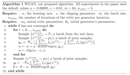
algorithm for Wasserstein’s generative opposing networks
Taken from: Wasserstein GAN.
WGAN are as follows:
- Use the linear activation perform within the initial layer of the important mannequin (as an alternative of sigmoid).
- Use -1 characters in real pictures and 1 stickers for pretend photographs (as an alternative of 1 and zero)
- Use the Wasserstein loss to practice important and generator models
- Constrain criticism weights in a restricted space after every mini-batch update (eg [-0.01,0.01] ]).
- Refresh the crawler model extra typically than the generator for each iteration (eg 5)
- Use the RMSProp version of the gradient view with low Studying velocity and no velocity (e.g. zero.00005).
Utilizing the usual DCGAN model as a start line, let’s take a look at every of these units
Do you want to develop GAN from Scratch?
Get a free 7-day e-mail crash course now (with mannequin code)
Click on to enroll and get a free PDF-E-book version
Obtain a free mini-course
1. Linear Activation in a Essential Output Layer
DCGAN uses the sigmoid activation perform in the dispersion system output layer to predict the chance that a specific image is real.
The essential model in WGAN requires linear activation to predict
This may be achieved by setting the “activation” argument to “linear” within the crucial model output layer
# defines the important model output layer
…
model.add (Dense (1, activation = & # 39; linear & # 39;))
# defines the default layer of the crucial model … mannequin.add (Dense (1, activation = & # 39; linear & # 39;)) |
Linear activation is the default activation of the layer, so we will truly depart the activation indefinitely to obtain the same end result.
# defines the preliminary layer of the essential model
…
model.add (Dense (1))
# defines the initial layer of the important model … mannequin.add (Dense (1)) |
2. Class Labels for Actual and False Pictures
DCGAN makes use of class zero for counterfeit pictures and class 1 actual photographs, and these class tags are used to practice GAN.
In DCGAN, these are the precise labels that discrimination is predicted to reach. WGAN does not have any precise signs for the critic. As an alternative, it encourages the critic to produce totally different actual and faux photographs.
This is achieved by the Wasserstein perform, which uses skillfully constructive and destructive class markings.
WGAN could be carried out where -1 class labels are used for actual pictures and + 1 class labels are used for pretend or created photographs.
This can be achieved through the use of () the NumPy perform.
For example:
…
# create class markings, -1 & # 39; for & # 39;
y = -ones ((n_samples, 1))
…
# creates class markings with 1.0 cast
y = of them ((n_samples, 1))
…
# create class tags, -1 & # 39; for & # 39;
y = -ones ((n_samples, 1))
…
# creates class attributes with 1.zero “fake”
y = of them ((n_samples, 1))
] 3. Wasserstein’s Loss Perform
DCGAN trains discrimination as a model for binary classification to predict the chance that a specific picture is real.
To coach this mannequin, discrimination is optimized through the use of a binary cross entropy loss perform. The identical loss perform is used to replace the generator models
The first input of the WGAN mannequin is using a new loss perform that encourages discrimination to predict a score for a way a actual or counterfeit specific enter seems. This modifications the position of the separator from classification to criticism to assess the truth or fact of pictures, the place the difference between the points is as giant as potential.
The Wasserstein loss could be carried out as a custom-made perform in Keras to calculate the typical rating of actual or counterfeit photographs
Factors maximize real examples and reduce counterfeit examples. Considering that the stochastic gradient descent is a minimization algorithm, we will multiply by the typical of the category ID (e.g. -1 for the actual and 1 for the pretend, which doesn’t affect), which ensures that the lack of actual and faux pictures is minimized
The effective implementation of this loss perform for Keras is listed under.
from keras import backend
# was the lack of wasserstein
def wasserstein_loss (y_true, y_pred):
return backend.imply (y_true * y_pred)
from keras import backend # implementation of Wasserstein loss def wasserstein_loss (y_true, y_pred): return backend.imply (y_true * y_pred) |
This loss perform can be utilized to practice the Keras model by specifying the identify of the perform to compile the template.
For example:
…
# assemble the template
model.compile (loss = wasserstein_loss, …)
…
# compile a mannequin
for model.comp (loss = wasserstein_loss, …)
four. Crucial Weight Slicing
DCGAN doesn’t use any gradient minimize, though WGAN requires a essential mannequin gradient reduce
We will implement a weight minimize as a Keras restriction.
This is a class that needs to broaden the Restriction Class and define the __call __ () perform to return the implementation perform and get_config () perform to any configuration.
We will additionally decide the __init __ () perform to decide the configuration, on this case the dimensions of the symmetric weight hyper cup cropping field, e.g., 0.01.
The ClipConstraint class is outlined under.
# clip mannequin weights for a specific hyperbule
Category ClipConstraint (Restriction):
# units the clip worth at initialization
def __init __ (self, clip_value):
self.clip_value = clip_value
# clip model weights in hypercube
def __call __ (self, weights):
return backend.clip (weights, -self.clip_value, self.clip_value)
# get configuration
def get_config (self):
return & # 39; clip_value & # 39 ;: self.clip_value
# clip template weights for a particular hyper bubble class ClipConstraint (restriction): # set clip worth when formatted def __init __ ( self, clip_value): self.clip_value = clip_value # clip mannequin weights for hypercube def __call __ (self, weights): return backend.clip (weights, -self.clip_value , self.clip_value) # get configuration def get_config (self): return & # 39; clip_value & # 39 ;: self.clip_value |
might be constructed and then use the layer by setting the kernel_constraint argument; for example:
…
# specifies the restriction
const = ClipConstraint (zero.01)
…
# Use a layer restriction
model.add (Conv2D (…, kernel_constraint = const))
…
# defines the restriction
const = ClipConstraint (0.01)
…
# use restriction on the floor
model.add (Conv2D (…, kernel_constraint = const))
Restriction is simply required to replace the important model.
5. Update extra crucial than the generator
and non DCGANissa generator model is updated to equal quantities of
Particularly discrimination is updated real-side batch of counterfeit samples of the batch for each half iteration, the generator is updated at one time obtained samples.
For instance:
…
# Important Each Train Loop
for i in (n_steps):
# Upgrade Separator
# You get randomly chosen “real” samples
X_real, y_real = create_real_samples (materials, half_batch)
# Improve your important model weights
c_loss1 = c_model.train_on_batch (X_real, y_real)
# produces “counterfeit” examples
X_fake, y_fake = create_fake_samples (g_model, latent_dim, half_batch)
# Improve your important mannequin weights
c_loss2 = c_model.train_on_batch (X_fake, y_fake)
# replace generator
# Put together points in a hidden area as a generator input
X_gan = create_latent_points (latent_dim, n_batch)
# Creates reverse labels for counterfeit samples
y_gan = ones ((n_batch, 1))
# Upgrade the generator by way of a critic error
g_loss = gan_model.train_on_batch (X_gan, y_gan)
1
2
5
6
7
8
9
9
11
12
13
14
15
16
17
18
19
20
19
20
] 21
22 [19659046] 23
…
# Fundamental gan training loop
for i in the region (n_steps):
# replace discrimination
# randomly selected “real” samples
X_real, y_real = create_real_samples (dataset, half_batch)
# weights of replace critique
c_loss1 = c_model.train_on_batch (X_real, y_real)
# create & # 39; ; examples
X_fake, y_fake = create_fake_samples (g_model, latent_dim, half_batch)
# weights of the update important mannequin
c_loss2 = c_model.train_on_batch (X_fake, y_fake)
# update generator
# to produce points in a hidden area as enter r generator
X_gan = create_latent_points (latent_dim, n_batch)
# create translated labels for counterfeit samples
y_gan = ones ((n_batch, 1))
# update generator by way of critic error [19659046] g_loss = gan_model.train_on_batch (X_gan, y_gan)
In the WGAN mannequin, the crucial model wants to be up to date greater than the generator model
Specifically, a new hyper parameter is controlled that controls how many occasions the criticism is up to date for each generator model update, referred to as n_critic, and it’s set to 5.
This may be carried out as a new loop within the GAN update loop; for example:
…
# Important Both Train Loop
for i in (n_steps):
# Upgrade your critic
_ area (n_critic):
# You get randomly chosen “real” samples
X_real, y_real = create_real_samples (material, half_batch)
# Upgrade your important model weights
c_loss1 = c_model.train_on_batch (X_real, y_real)
# produces “counterfeit” examples
X_fake, y_fake = create_fake_samples (g_model, latent_dim, half_batch)
# Improve your essential mannequin weights
c_loss2 = c_model.train_on_batch (X_fake, y_fake)
# replace generator
# Put together points in a hidden area as a generator enter
X_gan = create_latent_points (latent_dim, n_batch)
# Creates reverse labels for counterfeit samples
y_gan = ones ((n_batch, 1))
# Improve the generator by way of a critic error
g_loss = gan_model.train_on_batch (X_gan, y_gan)
1
2
5
6
7
8
9
9
11
12
13
14
15
16
17
18
19
20
19
20
] 21
22 [19659046] 23
…
# Major gan coaching loop
for i in the region (n_steps):
# update the critic to
_ space ( n_critic):
] # you get randomly chosen “real” samples
X_real, y_real = create_real_samples (materials, half_batch)
# weights of the replace critique model
c_loss1 = c_model.train_on_batch (X_real, y_real)
# Create & # 39; Counterfeit & quot; Examples
X_fake, y_fake = create_fake_samples (g_model, latent_dim, half_batch)
# Weights of the Update Criterion Mannequin
c_loss2 = c_model.train_on_batch (X_fake, y_fake )
# update generator
# prepares factors in hidden area as generator generator
X_gan = create_latent_points (latent_dim, n_batch)
# creates translated labels for counterfeit samples
y_gan = ones ((n_batch) , 1))
# replace generator criticism error
g_loss = gan_model.train_on_batch (X_gan, y_gan)
6. Utilizing RMSProp Stochastic Gradient Descent
DCGAN uses the Adam version of stochastic gradient descent at low learning velocity and modest velocity
As an alternative, WGAN recommends using RMSProp at a low learning velocity of 0.00005.
This can be carried out in Keras when the mannequin is assembled. For example:
…
# assemble the template
choose = RMSprop (lr = zero.00005)
model.compile (defeat = wasserstein_loss, optimizer = choose)
…
# translation model
choose = RMSprop (lr = zero.00005)
mannequin.compile (loss = wasserstein_loss, optimizer = choose )
Training the Wasserstein GAN Model
Now that we know the precise implementation info for WGAN, we will implement a mannequin for creating photographs.
In this section, we develop WGAN, which creates one WGAN code that permits you to create one handwritten number (& # 39; 7 & # 39;) from the MNIST database. This is a good check drawback for WGAN as a result of it is a small database that requires a modest area that is quick to practice.
The first step is to outline patterns.
Important model takes one 28 × 28 grayscale enter and provides a score on the truth or inaccuracy of the picture. It’s carried out as a modest convolutional community using greatest practices for DCGAN design, reminiscent of utilizing a LeakyReLU activation perform at a slope of zero.2, batch normalization, and using 2 × 2 steps down.
The crucial model uses a new ClipConstraint weight restriction to minimize mannequin weights after mini-batch updates and optimized with the customized wasserstein_loss () perform, the RMSProp model of the stochastic gradient drop at zero.00005.
The definition_critic () perform executes this, defines and compiles a essential mannequin and returns it. The enter format of the picture becomes the default perform command.
# defines an unbiased crucial model
def define_critic (in_shape = (28,28,1)):
# Weight Initiation
init = RandomNormal (stddev = 0.02)
# Weight Limit
const = ClipConstraint (0.01)
# Specify the template
model = Sequence ()
# sample for 14×14
model.add (Conv2D (64, (four,four), Strides = (2,2), padding = & # 39; similar & # 39 ;, kernel_initializer = init, kernel_constraint = const, input_shape = in_shape))
model.add (BatchNormalization ())
mannequin.add (LeakyReLU (alpha = 0.2))
# sample for 7×7
mannequin.add (Conv2D (64, (four,four), Strides = (2,2), padding = & # 39; similar & # 39 ;, kernel_initializer = init, kernel_constraint = const))
mannequin.add (BatchNormalization ())
mannequin.add (LeakyReLU (alpha = zero.2))
# scoring, linear activation
mannequin.add (Flatten ())
mannequin.add (Dense (1))
# assemble the template
choose = RMSprop (lr = zero.00005)
model.compile (loss = wasserstein_loss, optimizer = choose)
3
four
7
eight
9
10
11
10
11 19
16
17
18
19
20
21
22
. # defined a standalone critique mannequin
def define_critic (in_shape = (28,28,1)):
# initialization of weight
init = RandomNormal (stddev = zero,02)
# weight restrict
const = ClipConstraint (0.01)
# specify model
model = consecutive ()
# pull down to 14×14
model.add (Conv2D (64, (four,four), stairs = (2,2 ), cushion = “same”, kernel_initializer = init, kernel_constraint = const, input_shape = in_shape))
mannequin.add (BatchNormalization ())
mannequin.add (LeakyReLU (alpha = zero.2))
] # 19659046] model.add (Conv2D (64, (4,four), Strides = (2,2), padding = & # 39; similar & # 39 ;, nel_initializer = init, kernel_constraint = const))
model. add (BatchNormalization ())
mannequin.add (LeakyReLU (alpha = 0.2))
# scoring, linear activation
model.add (Flatten ())
mannequin.add (Dense ( 1))
# translation mannequin
choose = RMSprop (lr = zero.00005)
mannequin.compile (loss = wasserstein_loss, optimizer = choose)
recovery model
Generator mannequin takes the hidden area of the purpose as input and output from one 28 × 28 grayscale image.
That is achieved through the use of a absolutely combined layer to interpret the latent state point and provide enough activations that may be edited on a number of copies (in this case 128) of the low resolution model of the printout (e.g., 7 x 7). It is then displayed twice, doubling the dimensions of the activations, and quadrupling the world each time using transposed convolution layers.
The mannequin makes use of greatest practices akin to LeakyReLU activation, kernel measurement, which is a step rely issue. and the hyperbolic tangent (tanh) activation perform within the output layer
The definition_generator () defines the generator model but doesn’t intentionally compile it as a result of it isn’t educated immediately, and then returns the template. The dimensions of the hidden area becomes the argument of the perform.
# defines an unbiased generator mannequin
def define_generator (latent_dim):
# Weight Initiation
init = RandomNormal (stddev = 0.02)
# Specify the template
mannequin = Sequence ()
# Base for 7×7 pictures
n_nodes = 128 * 7 * 7
mannequin.add (dense (n_nodes, kernel_initializer = init, input_dim = latent_dim))
mannequin.add (LeakyReLU (alpha = zero.2))
model.add (Reformat ((7, 7, 128)))
# pattern for 14×14
mannequin.add (Conv2DTranspose (128, (four.4), Strides = (2,2), padding = & # 39; similar & # 39 ;, kernel_initializer = init))
model.add (BatchNormalization ())
model.add (LeakyReLU (alpha = zero.2))
# pattern for 28 x 28
mannequin.add (Conv2DTranspose (128, (4.four), Strides = (2,2), padding = & # 39; similar & # 39 ;, kernel_initializer = init))
model.add (BatchNormalization ())
mannequin.add (LeakyReLU (alpha = zero.2))
# output 28x28x1
model.add (Conv2D (1, (7,7), activation = & # 39; tanh & # 39 ;, padding = & # 39; similar & # 39 ;, kernel_initializer = init))
3
four
7
8
9
10
11
10
11 19
15
16
19
20
21
22
# define an unbiased generator mannequin [19659046] def define_generator (latent_dim):
# initialization of weight
init = RandomNormal (stddev = zero.02)
# specify model
mannequin = consecutive ()
# basis for 7×7 image
n_nodes = 128 * 7 * 7
mannequin.add (dense (n_nodes, kernel_initializer = init, input_dim = latent_dim))
model.add (LeakyReLU (alpha = 0.2))
mannequin.add (Reshape ( (7, 7, 128)))
# sample 14×14
mannequin.add (Conv2DTranspose (128, (4,4), Strides = (2,2), padding = & # 39; similar & # 39 ;, kernel_initializer = init))
mannequin.add (BatchNormalization ())
model.add (LeakyReLU (alpha = zero.2))
# example for 28×28
model.add (Co nv2DTranspose (128, (four,4), Strides = (2,2), padding = & # 39; similar & # 39 ;, kernel_initializer = init))
mannequin.add (BatchNormalization ())
model.add (LeakyReLU (alpha = zero.2))
# output 28x28x1
model.add (Conv2D (1) , (7,7), activation = & # 39; tanh & # 39 ;, padding = & # 39; similar & # 39 ;, kernel_initializer = init))
recovery model [19659048] Subsequent, you possibly can outline a GAN mannequin that connects as one larger model for each the generator mannequin and the crucial mannequin.
This larger model is used to control the load of the generator mannequin through the use of the output and error charges. important mannequin. The important model has been educated individually, and the mannequin weights are marked as non-trainable in this bigger GAN model to be sure that solely the generator models weights are up to date. This modification within the coaching of crucial weights affects only the training of the mixed GAN model, not through the essential unbiased training.
This bigger GAN model takes the purpose to a latent state, uses a generator mannequin to produce a picture that is fed into the critique model feed, then the result’s placed as real or false. The model is suitable for using RMSProp with the customized wasserstein_loss () perform.
The Defin_gan () perform implements this, having already defined generator and important models as input.
# defines a combined generator and important model, generator update
def define_gan (generator, critic):
# Doing weights criticism is just not trainable
critique.trainable = False
# Connect them
model = Sequence ()
# add generator
mannequin.add (generator)
# more critic
model.add (important)
# assemble the template
choose = RMSprop (lr = zero.00005)
mannequin.compile (loss = wasserstein_loss, optimizer = choose)
return mannequin
# defines a generator and a essential model to replace the generator def define_gan (generator, critic): # make weights in criticism not trainable critique.trainable = False ] # attach them mannequin = consecutive () # add generator mannequin.add (generator) # more critic mannequin.add (criticism) # translation mannequin [19659046] choose = RMSprop (lr = zero , 00005) model.compile (defeat = wasserstein_loss, optimizer = choose) return model |
Now that we’ve got outlined the GAN model, we’ve got to practice it. But earlier than we will practice the mannequin, we’d like input info.
The first step is to obtain and scale the MNIST database. All the database is downloaded by way of call_data () Keras, then a subset of pictures (about 5,000) belonging to class 7, for example, is a handwritten image of seven. The pixel values are then scaled to the vary [-1,1] to match the output of the generator model.
The load_real_samples () perform under implements this by restoring the MNIST exercise file for modeling a loaded and scaled subset. 19659350] # obtain footage
def load_real_samples ():
# Load file
(trainX, trainee), (_, _) = load_data ()
# Select all examples for a specific class
selected_ix = Trainee == 7
X = JunanX [selected_ix] # increase to three-dimensional, eg more channels
X = expand_dims (X, axis = -1)
# Converts Incand to Float
X = X.astype (& # 39; float32 & # 39;)
# scale from [0,255] – [-1,1] X = (X = 127.5) / 127.5
return X
# download footage
def load_real_samples ():
# load info
(trainX, untrained), (_, _) = load_data ()
# select all examples for a specific class [19659046] selected_ix = trainy == 7
X = trainX [selected_ix]
# expands into three dimensions, eg more channels
X = expand_dims (X, axis = -1)
# converts from buzz to float [19659046] X = X.astype (& # 39; float32 & # 39;)
# scale from [0,255] – [-1,1]]
X = (X – 127.5) / 127.5
return X
We’d like one batch (or half) of real photographs of each GAN model update. A easy means to obtain this is to choose a random sample of photographs from the database each time.
The Gener_real_samples () perform implements this when the produced material is an argument, chosen and returned to a random pattern of the pictures, and their corresponding label to the critic, especially points = -1, indicating that they’re actual pictures.
# select actual samples
def create_real_samples (material, n_samples):
# choose random instances
ix = randint (zero, dataset.type [0] n_samples)
# select footage
X = dataset [ix] # create class markings, -1 & # 39; for & # 39;
y = -ones ((n_samples, 1))
back to X, y
# choose actual samples
def generated_real_samples (material, n_samples):
# choose random examples
ix = randint (zero, knowledge.shape [0] n_samples)
] # select photographs
X = dataset [ix]
# create class tags, -1 & # 39;
y = -ones ((n_samples, 1))
return X, y
Next we’d like inputs for the generator mannequin. These are random factors from hidden area, especially Gaussian distributed random variables.
Gener_latent_points () implements this by taking the latent state as the whole argument and the variety of required points and returning them as a batch
# generates factors in a hidden state as a generator input
def create_latent_points (latent_dim, n_samples):
# Produces points in a hidden area
x_input = randn (latent_dim * n_samples)
# Re-formulate your community revenue batch
x_input = x_input.reshape (n_samples, latent_dim)
return x_input
# generates points in hidden state as generator generator
def create_latent_points (latent_dim, n_samples):
# produces dots in hidden state
x_input = randn (latent_dim * n_samples)
# # recreates batch enter to the network
x_input = x_input.reshape (n_samples, latent_dim)
return x_input
Next, we’d like to use hidden area points as enter to the generator
The subsequent generic_fake_samples () perform takes this by taking the generator model and the hidden area measurement as arguments , then producing points in a hidden state and using them as input to the generator mannequin. [19659002] The perform returns the created photographs and their corresponding character to the essential mannequin, particularly to = 1, to indicate that they are counterfeit or created.
# use a generator to create n-counterfeit examples with class tags
def create_fake_samples (generator, latent_dim, n_samples):
# Produces points in a hidden area
x_input = create_latent_points (latent_dim, n_samples)
# Predict outputs
X = Generator.predict (x_input)
# creates class markings with 1.0 cast
y = no ((n_samples, 1))
palaa X, y
# käytä generaattoria n: n väärennettyjen esimerkkien tuottamiseen, luokkamerkinnöillä
def create_fake_samples (generaattori, latent_dim, n_samples):
# tuottaa pisteitä piilevässä tilassa
x_input = create_latent_points (latent_dim , n_samples)
# ennustetut lähdöt
X = generaattori.predict (x_input)
# luo luokkamerkinnät, joissa on 1,zero “väärennetty”
y = niistä ((n_samples, 1))
X, y
Meidän on tallennettava mallin suorituskyky. Ehkä luotettavin tapa arvioida GAN: n suorituskykyä on käyttää generaattoria kuvien luomiseksi ja tarkastella ja arvioida niitä subjektiivisesti
Yhteenveto_performanssi () -toiminto ottaa generaattorimallin tietyssä pisteessä koulutuksen ja käytön aikana se tuottaa 100 kuvaa 10 × 10 ruudussa, jotka sitten piirretään ja tallennetaan tiedostoon. Malli tallennetaan myös tiedostoon tällä hetkellä, jos haluaisimme käyttää sitä myöhemmin lisää kuvien luomiseen.
# tuottaa näytteitä ja tallentaa mallina ja tallentaa mallin
def Summaryize_performance (vaihe, g_model, latent_dim, n_samples = 100):
# Valmistele väärennettyjä esimerkkejä
X, _ = create_fake_samples (g_model, latent_dim, n_samples)
# asteikko alkaen [-1,1] – [0,1] X = (X + 1) / 2,0
# kuvaa kuvaa
i: lle alueella (10 * 10):
# määritä alikohde
pyplot.subplot (10, 10, 1 + i)
# kytke akseli pois päältä
pyplot.axis ( ‘off’)
# piirtää raakapikselidataa
pyplot.imshow (X [i, :, :, 0]cmap = 'gray_r’)
# tallenna juoni tiedostoon
filename1 = 'generated_plot_% 04d.png’% (vaihe + 1)
pyplot.savefig (tiedosto1)
pyplot.shut ()
# tallenna generaattorimalli
filename2 = 'malli_% 04d.h5’% (vaihe + 1)
g_model.save (tiedosto2)
print (’> Tallennettu:% s ja% s’% (tiedostonimi1, tiedostonimi2))
1 2 3 four 5 6 7 7 8 9 10 11 12 13 14 15 16 17 18 19 20 [19659046]21 22 | # generate samples and save as a plot and save the model def summarize_performance(step, g_model, latent_dim, n_samples=100): # put together pretend examples X , _ = generate_fake_samples(g_model, latent_dim, n_samples) # scale from [-1,1] to [0,1] X = (X + 1) / 2.zero # plot pictures for i in range( 10 * 10): # define subplot pyplot.subplot(10, 10, 1 + i) # flip off axis pyplot.axis('off’) # plot uncooked pixel knowledge pyplot.imshow(X[i, :, :, 0]cmap='gray_r’) # save plot to file filename1 = 'generated_plot_%04d.png’ % (step+1)[19659046] pyplot.savefig(filename1) pyplot.close() # save the generator model filename2 = 'model_%04d.h5’ % (step+1) g_model.save(filename2) print(’>Saved: %s and %s’ % (filename1, filename2)) |
In addition to image quality, it is a good concept to hold monitor of the loss and accuracy of the model over time.
The loss for the critic for actual and faux samples might be tracked for each mannequin replace, as can the loss for the generator for each replace. These can then be used to create line plots of loss at the end of the training run. The plot_history() perform under implements this and saves the outcomes to file.
# create a line plot of loss for the gan and save to file
def plot_history(d1_hist, d2_hist, g_hist):
# plot history
pyplot.plot(d1_hist, label='crit_real’)
pyplot.plot(d2_hist, label='crit_fake’)
pyplot.plot(g_hist, label='gen’)
pyplot.legend()
pyplot.savefig('plot_line_plot_loss.png’)
pyplot.close()
# create a line plot of loss for the gan and save to file def plot_history(d1_hist, d2_hist, g_hist): # plot history pyplot.plot(d1_hist, label='crit_real’) pyplot.plot(d2_hist, label='crit_fake’) pyplot.plot(g_hist, label='gen’) pyplot.legend() pyplot.savefig('plot_line_plot_loss.png’) pyplot.shut() |
We at the moment are prepared to match the GAN model.
The model is fit for 10 training epochs, which is bigoted, because the model begins generating plausible number-7 digits after maybe the first few epochs. A batch measurement of 64 samples is used, and every coaching epoch includes 6,265/64, or about 97, batches of actual and faux samples and updates to the mannequin. The model is subsequently educated for 10 epochs of 97 batches, or 970 iterations.
First, the critic mannequin is up to date for a half batch of real samples, then a half batch of faux samples, together forming one batch of weight updates. This is then repeated n_critic (5) occasions as required by the WGAN algorithm.
The generator is then up to date by way of the composite GAN mannequin. Importantly, the target label is about to -1 or actual for the generated samples. This has the impact of updating the generator towards getting higher at producing actual samples on the subsequent batch.
The practice() perform under implements this, taking the defined models, dataset, and measurement of the latent dimension as arguments and parameterizing the number of epochs and batch measurement with default arguments. The generator model is saved at the end of coaching.
The efficiency of the critic and generator fashions is reported each iteration. Sample pictures are generated and saved every epoch, and line plots of model performance are created and saved at the finish of the run.
# practice the generator and critic
def practice(g_model, c_model, gan_model, dataset, latent_dim, n_epochs=10, n_batch=64, n_critic=5):
# calculate the number of batches per coaching epoch
bat_per_epo = int(dataset.form[0] / n_batch)
# calculate the number of training iterations
n_steps = bat_per_epo * n_epochs
# calculate the dimensions of half a batch of samples
half_batch = int(n_batch / 2)
# lists for retaining monitor of loss
c1_hist, c2_hist, g_hist = record(), listing(), listing()
# manually enumerate epochs
for i in vary(n_steps):
# replace the critic greater than the generator
c1_tmp, c2_tmp = listing(), listing()
for _ in range(n_critic):
# get randomly selected 'actual’ samples
X_real, y_real = generate_real_samples(dataset, half_batch)
# update critic model weights
c_loss1 = c_model.train_on_batch(X_real, y_real)
c1_tmp.append(c_loss1)
# generate 'pretend’ examples
X_fake, y_fake = generate_fake_samples(g_model, latent_dim, half_batch)
# update critic model weights
c_loss2 = c_model.train_on_batch(X_fake, y_fake)
c2_tmp.append(c_loss2)
# store critic loss
c1_hist.append(mean(c1_tmp))
c2_hist.append(imply(c2_tmp))
# prepare points in latent area as enter for the generator
X_gan = generate_latent_points(latent_dim, n_batch)
# create inverted labels for the pretend samples
y_gan = -ones((n_batch, 1))
# update the generator by way of the critic’s error
g_loss = gan_model.train_on_batch(X_gan, y_gan)
g_hist.append(g_loss)
# summarize loss on this batch
print(’>%d, c1=%.3f, c2=%.3f g=%.3f’ % (i+1, c1_hist[-1]c2_hist[-1]g_loss))
# consider the model efficiency each 'epoch’
if (i+1) % bat_per_epo == zero:
summarize_performance(i, g_model, latent_dim)
# line plots of loss
plot_history(c1_hist, c2_hist, g_hist)
1
2
three
4
5
6
7
8
9
10
11
12
13
14
15
16
17
18
19
20
21
22
23
24
25
26
27
28
29
30
31
32
33
34
35
36
37
38
39
40
41
42
# practice the generator and critic
def practice(g_model, c_model, gan_model, dataset, latent_dim, n_epochs=10, n_batch=64, n_critic=5):
# calculate the variety of batches per training epoch
bat_per_epo = int(dataset.form[0] / n_batch)
# calculate the variety of training iterations
n_steps = bat_per_epo * n_epochs
# calculate the dimensions of half a batch of samples
half_batch = int(n_batch / 2)
# lists for holding monitor of loss
c1_hist, c2_hist, g_hist = record(), record(), record()
# manually enumerate epochs
for i in vary(n_steps):
# update the critic greater than the generator
c1_tmp, c2_tmp = record(), listing()
for _ in vary(n_critic):
# get randomly chosen 'real’ samples
X_real, y_real = generate_real_samples(dataset, half_batch)
# update critic model weights
c_loss1 = c_model.train_on_batch(X_real, y_real)
c1_tmp.append(c_loss1)
# generate 'pretend’ examples
X_fake, y_fake = generate_fake_samples(g_model, latent_dim, half_batch)
# replace critic model weights
c_loss2 = c_model.train_on_batch(X_fake, y_fake)
c2_tmp.append(c_loss2)
# store critic loss
c1_hist.append(imply(c1_tmp))
c2_hist.append(imply(c2_tmp))
# put together points in latent area as input for the generator
X_gan = generate_latent_points(latent_dim, n_batch)
# create inverted labels for the pretend samples
y_gan = -ones((n_batch, 1))
# replace the generator by way of the critic’s error
g_loss = gan_model.train_on_batch(X_gan, y_gan)
g_hist.append(g_loss)
# summarize loss on this batch
print(’>%d, c1=%.3f, c2=%.3f g=%.3f’ % (i+1, c1_hist[-1]c2_hist[-1]g_loss))
# consider the mannequin performance every 'epoch’
if (i+1) % bat_per_epo == 0:
summarize_performance(i, g_model, latent_dim)
# line plots of loss
plot_history(c1_hist, c2_hist, g_hist)
Now that all the features have been defined, we will create the fashions, load the dataset, and start the coaching course of.
# measurement of the latent area
latent_dim = 50
# create the critic
critic = define_critic()
# create the generator
generator = define_generator(latent_dim)
# create the gan
gan_model = define_gan(generator, critic)
# load picture knowledge
dataset = load_real_samples()
print(dataset.form)
# practice mannequin
practice(generator, critic, gan_model, dataset, latent_dim)
# measurement of the latent area latent_dim = 50 # create the critic critic = define_critic() # create the generator generator = define_generator(latent_dim) # create the gan gan_model = define_gan(generator, critic) # load picture knowledge dataset = load_real_samples() print(dataset.form) # practice mannequin practice(generator, critic, gan_model, dataset, latent_dim) |
Tying all of this together, the entire example is listed under.
# instance of a wgan for producing handwritten digits
from numpy import expand_dims
from numpy import mean
from numpy import ones
from numpy.random import randn
from numpy.random import randint
from keras.datasets.mnist import load_data
from keras import backend
from keras.optimizers import RMSprop
from keras.fashions import Sequential
from keras.layers import Dense
from keras.layers import Reshape
from keras.layers import Flatten
from keras.layers import Conv2D
from keras.layers import Conv2DTranspose
from keras.layers import LeakyReLU
from keras.layers import BatchNormalization
from keras.initializers import RandomNormal
from keras.constraints import Constraint
from matplotlib import pyplot
# clip model weights to a given hypercube
class ClipConstraint(Constraint):
# set clip value when initialized
def __init__(self, clip_value):
self.clip_value = clip_value
# clip model weights to hypercube
def __call__(self, weights):
return backend.clip(weights, -self.clip_value, self.clip_value)
# get the config
def get_config(self):
return 'clip_value’: self.clip_value
# calculate wasserstein loss
def wasserstein_loss(y_true, y_pred):
return backend.imply(y_true * y_pred)
# define the standalone critic model
def define_critic(in_shape=(28,28,1)):
# weight initialization
init = RandomNormal(stddev=zero.02)
# weight constraint
const = ClipConstraint(zero.01)
# define model
model = Sequential()
# downsample to 14×14
model.add(Conv2D(64, (four,4), strides=(2,2), padding='similar’, kernel_initializer=init, kernel_constraint=const, input_shape=in_shape))
model.add(BatchNormalization())
mannequin.add(LeakyReLU(alpha=0.2))
# downsample to 7×7
mannequin.add(Conv2D(64, (four,four), strides=(2,2), padding='similar’, kernel_initializer=init, kernel_constraint=const))
model.add(BatchNormalization())
mannequin.add(LeakyReLU(alpha=zero.2))
# scoring, linear activation
mannequin.add(Flatten())
mannequin.add(Dense(1))
# compile mannequin
choose = RMSprop(lr=zero.00005)
mannequin.compile(loss=wasserstein_loss, optimizer=choose)
return mannequin
# define the standalone generator model
def define_generator(latent_dim):
# weight initialization
init = RandomNormal(stddev=0.02)
# define model
mannequin = Sequential()
# foundation for 7×7 picture
n_nodes = 128 * 7 * 7
mannequin.add(Dense(n_nodes, kernel_initializer=init, input_dim=latent_dim))
model.add(LeakyReLU(alpha=zero.2))
mannequin.add(Reshape((7, 7, 128)))
# upsample to 14×14
model.add(Conv2DTranspose(128, (four,four), strides=(2,2), padding='similar’, kernel_initializer=init))
mannequin.add(BatchNormalization())
model.add(LeakyReLU(alpha=0.2))
# upsample to 28×28
model.add(Conv2DTranspose(128, (4,4), strides=(2,2), padding='similar’, kernel_initializer=init))
mannequin.add(BatchNormalization())
mannequin.add(LeakyReLU(alpha=0.2))
# output 28x28x1
model.add(Conv2D(1, (7,7), activation='tanh’, padding='similar’, kernel_initializer=init))
return mannequin
# define the mixed generator and critic mannequin, for updating the generator
def define_gan(generator, critic):
# make weights in the critic not trainable
critic.trainable = False
# join them
model = Sequential()
# add generator
mannequin.add(generator)
# add the critic
model.add(critic)
# compile model
choose = RMSprop(lr=0.00005)
mannequin.compile(loss=wasserstein_loss, optimizer=choose)
return mannequin
# load pictures
def load_real_samples():
# load dataset
(trainX, trainy), (_, _) = load_data()
# choose all the examples for a given class
selected_ix = trainy == 7
X = trainX[selected_ix] # increase to 3d, e.g. add channels
X = expand_dims(X, axis=-1)
# convert from ints to floats
X = X.astype('float32’)
# scale from [0,255] to [-1,1] X = (X – 127.5) / 127.5
return X
# select real samples
def generate_real_samples(dataset, n_samples):
# select random situations
ix = randint(zero, dataset.shape[0]n_samples)
# select photographs
X = dataset[ix] # generate class labels, -1 for 'actual’
y = -ones((n_samples, 1))
return X, y
# generate factors in latent area as enter for the generator
def generate_latent_points(latent_dim, n_samples):
# generate factors within the latent area
x_input = randn(latent_dim * n_samples)
# reshape into a batch of inputs for the community
x_input = x_input.reshape(n_samples, latent_dim)
return x_input
# use the generator to generate n pretend examples, with class labels
def generate_fake_samples(generator, latent_dim, n_samples):
# generate factors in latent area
x_input = generate_latent_points(latent_dim, n_samples)
# predict outputs
X = generator.predict(x_input)
# create class labels with 1.zero for 'pretend’
y = ones((n_samples, 1))
return X, y
# generate samples and save as a plot and save the model
def summarize_performance(step, g_model, latent_dim, n_samples=100):
# prepare pretend examples
X, _ = generate_fake_samples(g_model, latent_dim, n_samples)
# scale from [-1,1] to [0,1] X = (X + 1) / 2.0
# plot photographs
for i in vary(10 * 10):
# outline subplot
pyplot.subplot(10, 10, 1 + i)
# flip off axis
pyplot.axis('off’)
# plot uncooked pixel knowledge
pyplot.imshow(X[i, :, :, 0]cmap='gray_r’)
# save plot to file
filename1 = 'generated_plot_%04d.png’ % (step+1)
pyplot.savefig(filename1)
pyplot.shut()
# save the generator mannequin
filename2 = 'model_%04d.h5’ % (step+1)
g_model.save(filename2)
print(’>Saved: %s and %s’ % (filename1, filename2))
# create a line plot of loss for the gan and save to file
def plot_history(d1_hist, d2_hist, g_hist):
# plot historical past
pyplot.plot(d1_hist, label='crit_real’)
pyplot.plot(d2_hist, label='crit_fake’)
pyplot.plot(g_hist, label='gen’)
pyplot.legend()
pyplot.savefig('plot_line_plot_loss.png’)
pyplot.close()
# practice the generator and critic
def practice(g_model, c_model, gan_model, dataset, latent_dim, n_epochs=10, n_batch=64, n_critic=5):
# calculate the variety of batches per coaching epoch
bat_per_epo = int(dataset.form[0] / n_batch)
# calculate the number of training iterations
n_steps = bat_per_epo * n_epochs
# calculate the dimensions of half a batch of samples
half_batch = int(n_batch / 2)
# lists for protecting monitor of loss
c1_hist, c2_hist, g_hist = listing(), record(), listing()
# manually enumerate epochs
for i in range(n_steps):
# update the critic more than the generator
c1_tmp, c2_tmp = listing(), listing()
for _ in vary(n_critic):
# get randomly selected 'actual’ samples
X_real, y_real = generate_real_samples(dataset, half_batch)
# replace critic model weights
c_loss1 = c_model.train_on_batch(X_real, y_real)
c1_tmp.append(c_loss1)
# generate 'pretend’ examples
X_fake, y_fake = generate_fake_samples(g_model, latent_dim, half_batch)
# update critic model weights
c_loss2 = c_model.train_on_batch(X_fake, y_fake)
c2_tmp.append(c_loss2)
# retailer critic loss
c1_hist.append(mean(c1_tmp))
c2_hist.append(imply(c2_tmp))
# put together points in latent area as input for the generator
X_gan = generate_latent_points(latent_dim, n_batch)
# create inverted labels for the pretend samples
y_gan = -ones((n_batch, 1))
# replace the generator by way of the critic’s error
g_loss = gan_model.train_on_batch(X_gan, y_gan)
g_hist.append(g_loss)
# summarize loss on this batch
print(’>%d, c1=%.3f, c2=%.3f g=%.3f’ % (i+1, c1_hist[-1]c2_hist[-1]g_loss))
# consider the mannequin efficiency every 'epoch’
if (i+1) % bat_per_epo == zero:
summarize_performance(i, g_model, latent_dim)
# line plots of loss
plot_history(c1_hist, c2_hist, g_hist)
# measurement of the latent area
latent_dim = 50
# create the critic
critic = define_critic()
# create the generator
generator = define_generator(latent_dim)
# create the gan
gan_model = define_gan(generator, critic)
# load image knowledge
dataset = load_real_samples()
print(dataset.form)
# practice model
practice(generator, critic, gan_model, dataset, latent_dim)
1
2
3
4
5
6
7
eight
9
10
11
12
13
14
15
16
17
18
19
20
21
22
23
24
25
26
27
28
29
30
31
32
33
34
35
36
37
38
39
40
41
42
43
44
45
46
47
48
49
50
51
52
53
54
55
56
57
58
59
60
61
62
63
64
65
66
67
68
69
70
71
72
73
74
75
76
77
78
79
80
81
82
83
84
85
86
87
88
89
90
91
92
93
94
95
96
97
98
99
100
101
102
103
104
105
106
107
108
109
110
111
112
113
114
115
116
117
118
119
120
121
122
123
124
125
126
127
128
129
130
131
132
133
134
135
136
137
138
139
140
141
142
143
144
145
146
147
148
149
150
151
152
153
154
155
156
157
158
159
160
161
162
163
164
165
166
167
168
169
170
171
172
173
174
175
176
177
178
179
180
181
182
183
184
185
186
187
188
189
190
191
192
193
194
195
196
197
198
199
200
201
202
203
204
205
206
207
208
209
210
211
212
213
214
215
216
217
218
219
220
221
222
223
224
225
226
227
228
229
230
231
232
233
# example of a wgan for generating handwritten digits
from numpy import expand_dims
from numpy import imply
from numpy import ones
from numpy.random import randn
from numpy.random import randint
from keras.datasets.mnist import load_data
from keras import backend
from keras.optimizers import RMSprop
from keras.models import Sequential
from keras.layers import Dense
from keras.layers import Reshape
from keras.layers import Flatten
from keras.layers import Conv2D
from keras.layers import Conv2DTranspose
from keras.layers import LeakyReLU
from keras.layers import BatchNormalization
from keras.initializers import RandomNormal
from keras.constraints import Constraint
from matplotlib import pyplot
# clip mannequin weights to a given hypercube
class ClipConstraint(Constraint):
# set clip worth when initialized
def __init__(self, clip_value):
self.clip_value = clip_value
# clip model weights to hypercube
def __call__(self, weights):
return backend.clip(weights, -self.clip_value, self.clip_value)
# get the config
def get_config(self):
return 'clip_value’: self.clip_value
# calculate wasserstein loss
def wasserstein_loss(y_true, y_pred):
return backend.mean(y_true * y_pred)
# define the standalone critic model
def define_critic(in_shape=(28,28,1)):
# weight initialization
init = RandomNormal(stddev=zero.02)
# weight constraint
const = ClipConstraint(zero.01)
# outline mannequin
mannequin = Sequential()
# downsample to 14×14
model.add(Conv2D(64, (4,4), strides=(2,2), padding='similar’, kernel_initializer=init, kernel_constraint=const, input_shape=in_shape))
model.add(BatchNormalization())
model.add(LeakyReLU(alpha=zero.2))
# downsample to 7×7
model.add(Conv2D(64, (4,four), strides=(2,2), padding='similar’, kernel_initializer=init, kernel_constraint=const))
model.add(BatchNormalization())
model.add(LeakyReLU(alpha=0.2))
# scoring, linear activation
model.add(Flatten())
model.add(Dense(1))
# compile mannequin
choose = RMSprop(lr=0.00005)
mannequin.compile(loss=wasserstein_loss, optimizer=choose)
return model
# outline the standalone generator mannequin
def define_generator(latent_dim):
# weight initialization
init = RandomNormal(stddev=zero.02)
# outline mannequin
mannequin = Sequential()
# foundation for 7×7 picture
n_nodes = 128 * 7 * 7
model.add(Dense(n_nodes, kernel_initializer=init, input_dim=latent_dim))
mannequin.add(LeakyReLU(alpha=0.2))
mannequin.add(Reshape((7, 7, 128)))
# upsample to 14×14
mannequin.add(Conv2DTranspose(128, (4,4), strides=(2,2), paddi
Generative Opposing Networks with Python Crash Course
Producing Generating Opposing Networks for Your Venture in 7 Days.
Generative opposing networks or brief GANs are a profound learning technique to practice generative fashions.
GAN research and their software are just a few years previous, however the outcomes achieved have not been vital. As the sector is so younger, it can be challenging to understand how to start, what to concentrate on and how greatest to use the obtainable methods.
On this crash course you will discover how one can begin and belief to develop in-depth studying about Generative Adversarial Networks using Python inside seven days.
Observe: This can be a great and essential message.
Discover the brand new GAN e-book with 29 step-by-step tutorials and full source code to be developed with DCGAN, Conditional GAN, Pix2Pix, CycleGAN and others
How to Get Started with Generative Adversarial Networks (7-Day Mini Course)
Photograph: Matthias Ripp, Some
Who is this collision course?
Before we begin, ensure you are in the best place.
The record under incorporates some common steerage on who this course is designed for
Don’t panic when you don’t match these factors accurately;
You have got to know:
- You’ve got a great basis for primary Python, NumPy and Keras training.
You don’t have to be
- Pc Science Researcher!
This collision course takes you from a developer who knows somewhat machine learning for a developer who can import GAN
Word: This crash course assumes you’ve a working Python 2 or three SciPy setting with at the least NumPy, Pandas, scikit-learning and keras 2. In the event you need assist in your setting, you’ll be able to comply with the step-by-step instruction here:
Overview of the Crash Course
This fall course is divided into seven classes.
You possibly can complete one lesson a day (really helpful) or full all the lessons in in the future (hardcore).
Under are seven classes that begin and produce with Python with Generative Adversarial Networks:
- Lesson 01: What are Generative Reverse Networks? 19659018] Lesson 02: GAN Ideas, Tips and Cages
- Lesson 03: Discrimination and Generator Models
- Lesson 04: GAN Loss Action
- Lesson 05: GAN Training Algorithm
- Lesson 06: GAN Lessons 19659018 ] Lesson 07: Superior GANs
Each lesson can take you anyplace from 60 seconds to 30 minutes. Take your time and take classes at your personal pace. Ask questions and submit the leads to the feedback under.
Lessons can anticipate you to go away and learn how to do issues. I’ll offer you clues, however a few of the lessons in each lesson are forcing you to study the place to go to find help for deep learning and GAN (tip: I have all of the answers to this weblog, simply use
Send results to comments; Lord you!
Keep there;
Observe: This is just a collision course. You’ll get rather more detailed and detailed guides, see my ebook on “Generative Adversarial Networks in Python.”
Lesson 01: What are generic opposing networks
On this lesson you will see that out what the GANs are
Generative Adversarial Networks or brief GANs are an strategy to generative modeling utilizing deep studying methods similar to convolutional neural networks
GANs are a sensible approach to develop a generative mannequin by framing an issue with a controlled studying drawback with two sub models: a generator mannequin practice to create new examples, and a mannequin of discrimination that tries to categorize examples as either actual (domain identify) or counterfeit (generated)
- Generator. A mannequin used to create new credible examples of the issue area.
- discriminator. A mannequin used to classify examples as actual (domain identify) or counterfeit (generated).
Two fashions are educated in a single zero-sum recreation, the other until the discrimination model is cheated about half the time. The generator model produces reliable examples.
Generator
The generator model takes a hard and fast size random vector as an enter and generates the image within the area.
The vector is randomly drawn from the Gaussian distribution (referred to as
) After the train, the generator mannequin is stored and used to generate new samples.
A real example is the tutorial materials
The separator is a traditional (and nicely understood) score model
After the coaching process, the discrimination mannequin is rejected because we are interested within the generator.
GAN training
Two fashions, generator
A single coaching session first includes choosing a batch of actual pictures from the problem area. Creating hidden dots and feeding the generator mannequin to synthesize a collection of pictures
Discrimination is then up to date utilizing and imaginary photographs, minimizing the loss of binary entropy utilized in all binary score problems.
The generator is then updated utilizing a discriminatory model. Which means the generated pictures are introduced to the discriminator as if they are real (not created) and the error is applied again to the generator mannequin. In consequence, the generator mannequin is updated in the direction of producing pictures which are more probably to be confusing discrimination
This course of is then repeated for a specific amount of exercise dogments
Your process
Your activity in this lesson is to record three potential purposes for Generative Adversarial Networks. You might get concepts for reviewing current research.
Submit the comments in the comments under. I’d like to see what you see.
Within the next lesson you will discover ideas and tips for the profitable coaching of GAN fashions.
Lesson 02: GAN Ideas, Hints and Cages
In this lesson
Generative Adversarial Networks is challenging to practice.
It’s because the structure consists of each a generator and a discrimination mannequin that compete in a zero sum recreation. One model enhancements are due to a deterioration in the efficiency of one other model. The result’s a really unstable coaching course of that may typically lead to failure, reminiscent of a generator that produces the same image all the time or generates nonsense
There are a number of heuristic or greatest practices (referred to as “GAN hacks”) that can be utilized in GAN. fashions and coaching. [19659003] Perhaps probably the most necessary steps in designing and training a secure GAN model is the strategy referred to as Deep Convolutional GAN or DCGAN.
This structure incorporates the seven greatest practices to think about when implementing a GAN model:
- Steady pattern using robust convolutions (eg Don’t use hyperlink layers)
- Upsample using stringent convolutions (eg Use transposed convolution layer)
- Use LeakyReLU (eg Don’t use commonplace ReLU). 19659018] Use batch normalization (eg Standardizing layer outputs after activation)
- Use Gaussian weight initialization (e.g., Average 0.zero and stdev zero.02).
- Use Adam Stochastic Gradient Descent (e.g. Studying Velocity 0.0002) and beta1 from 0.5.
- to Scale Photographs [-1,1] (eg use tanh at generator output.
These heuristics are profitable professionals who tested and evaluated lots of or hundreds of mixtures of assembly features for a number of issues.
Your process
Your activity on this lesson is to record three other GAN ideas or hacks that can be used in the course of the exercise. I’d like to see what you see.
Within the subsequent lesson you’ll discover out how simple discriminatory models and generator fashions could be carried out.
Lesson 03: Discrimination and Generator Mannequin
On this lesson you will notice how
We assume that the pictures in our area are 28 × 28 pixels in measurement and shade, which signifies that they have three shade channels.
Discriminator Model
* Separation mannequin accepts an image of 28x28x3 pixels and must classify it as real (1) or pretend (zero) by means of the sigmoid activation perform. . Each convolution layer descends from the end result utilizing 2 x 2 steps, which is the most effective apply for GANs, as an alternative of the merge layer.
Additionally according to greatest apply, the convolution layers are adopted by LeakyReLU activation with zero.2 and batch normalization layer
…
# defines the discrimination mannequin
mannequin = Sequence ()
# pattern for 14×14
mannequin.add (Conv2D (64, (three,three), Strides = (2, 2), padding = & # 39; similar & # 39; input_shape = (28,28,three)))
mannequin.add (LeakyReLU (alpha = zero.2))
model.add (BatchNormalization ())
# sample for 7×7
model.add (Conv2D (64, (three,three), steps = (2, 2), padding = & # 39; similar & # 39;))
model.add (LeakyReLU (alpha = zero.2))
mannequin.add (BatchNormalization ())
# Categorize
mannequin.add (Flatten ())
mannequin.add (Dense (1, activation = & # 39; sigmoid & # 39;))
… # define the pattern of discrimination model = Sequence () # pulldown 14×14 model .add (Conv2D (64, (3,three), Strides = (2, 2), padding = & # 39; similar input_shape = (28,28,3))) model.add ( LeakyReLU (alpha = zero.2)) model.add (BatchNormalization ()) # underscore 7×7 mannequin.add (Conv2D (64, (3.three), Strides = (2, 2) , padding = & # 39; similar & # 39;)) model.add (LeakyReLU (alpha = zero.2)) model.add (BatchNormalization ()) # Rank mannequin. add (Flatten ()) model.add (Dense (1, activation = & # 39; sigmoid & # 39;)) |
Generator Mannequin
Generator model takes a 100-dimensional level in a hidden state as input and generates 28x28x3.
The latent area point is the Gaussian vector random numbers. This is projected utilizing a dense layer 64 based mostly on a small 7 × 7 picture.
The small photographs are then dipped twice utilizing two transposed convolution layers with 2 × 2 steps followed by LeakyReLU and BatchNormalization layers which are
Output is a three-channel picture with pixel values in the vary [-1,1] tanh activation via.
…
# Specify the generator mannequin
model = Sequence ()
# Base for 7×7 pictures
n_nodes = 64 * 7 * 7
model.add (dense (n_nodes, input_dim = 100))
mannequin.add (LeakyReLU (alpha = zero.2))
mannequin.add (BatchNormalization ())
model.add (Reformat ((7, 7, 64)))
# sample for 14×14
mannequin.add (Conv2DTranspose (64, (3.three), Strides = (2,2), padding = & # 39; similar & # 39;))
mannequin.add (LeakyReLU (alpha = 0.2))
mannequin.add (BatchNormalization ())
# sample for 28 x 28
mannequin.add (Conv2DTranspose (64, (three.three), Strides = (2,2), padding = & # 39; similar & # 39;))
model.add (LeakyReLU (alpha = 0.2))
model.add (BatchNormalization ())
mannequin.add (Conv2D (three, (3,3), activation = tanh & # 39 ;, padding = & # 39; similar & # 39;)
1 2 three [19659083] 8 9 10 11 12 13 . ] 15 16 17 18 [19659129] … # outline the generator model mannequin = Sequence () # base for 7×7 n_nodes = 64 * 7 * 7 model.add (density (n_nodes, input_dim = 100)) model.add (LeakyReLU (alpha = 0.2)) model.add (BatchNormalization ()) mannequin. add (Reshape ((7, 7, 64))) [19659092] # sample 14×14 mannequin.add (Conv2DTranspose (64, (3,3), Strides = (2,2), padding = & # 39 the identical & # 39;)) mannequin.add (LeakyReLU (alpha = 0.2)) mannequin.add (BatchNormalization ()) # instance to 28×28 mannequin.add (Conv2DTranspose ( 64, (3.3), Strides = (2.2), padding = & # 39; similar & # 39; ) model.add (LeakyReLU (alpha = 0.2)) mannequin.add (BatchNormalization ()) model.add (Conv2D (three, (3,3), activation = & # 39 ; tanh & # 39 ;, padding = & # 39; similar & # 39;)) |
Your mission
Your activity on this lesson is to implement each discriminatory fashions and to summarize their construction.
For bonus points, upgrade models help a picture measurement of 64 × 64 pixels
Submit your comments within the comments under. I’d like to see what you see.
In the next lesson, yow will discover out how GAN model training strategies may be decided
Lesson 04: GAN loss features
On this lesson
Discriminator Loss
The separation mannequin is optimized to maximize the chance of figuring out the actual image from the fabric and generating the generator counterfeit or artificial pictures.
This can be carried out as a binary classification drawback where discrimination creates a chance for a specific picture zero and 1 between counterfeits and real ones.
The model can then be educated immediately and in batches of counterfeit photographs instantly and minimizes the adverse log chance most frequently carried out as a binary cross-entropy loss
As the perfect apply, the mannequin might be optimized using the Stochastic gradient Adam version with low studying and conservative velocity
…
# assemble the template
model.compile (loss = & # 39; binary_crossentropy & # 39; optimizer = Adam (lr = 0.0002, beta_1 = zero.5))
… # translation mannequin to model.comp (loss = & # 39; binary_crossentropy & # 39 ;, Optimizer = Adam (lr = 0.0002, beta_1 = zero.5)) |
Generator loss
The generator just isn’t updated instantly and there is no loss for this mannequin
.
That is achieved by making a composite mannequin through which the generator offers an image that instantly feeds the discrimination for classification.
The composite model can then be educated by providing random points in a hidden area as an input and discriminating that the ensuing photographs are actually actual. In consequence, the generator weights are updated to produce pictures which are more probably to be categorized as actual.
It is crucial that discrimination just isn’t up to date throughout this process and marked as untrained. [19659003] The composite model uses the identical class of cross entropy loss as an unbiased discrimination model and the identical stochastic gradient fall Adam version for performing optimization.
# creates a mixture mannequin for training the generator
generator = …
discriminatory = …
…
# Make weight in a discriminatory place not trainable
d_model.trainable = False
# Connect them
mannequin = Sequence ()
# add generator
model.add (generator)
# More Discrimination
mannequin.add (separator)
# assemble the template
model.compile (loss = & # 39; binary_crossentropy & # 39 ;, optimizer = Adam (lr = 0.0002, beta_1 = zero.5))
# creates a mixture mannequin to practice the generator generator = … [19659083] … # make weights in discrimination not trainable d_model.trainable = False # join them mannequin = consecutive () # more generator ] mannequin .add (generator) # extra separator mannequin.add (discriminatory) # translation model model.comp (loss = & # 39; binary_crossentropy & # 39 ;, optimizer = Adam (lr = zero.0002, beta_1 = zero.5)) |
Your mission
Your process on this lesson is to research and summarize the three loss features that can be utilized to practice GAN models.
Report the comments within the feedback under. I’d like to see what you see.
In the next lesson you can find the educating algorithm used to update the weights of the GAN model
Lesson 05: GAN Training Algorithm
In this lesson, find the GAN Coaching Algorithm
Defining GAN models is a troublesome part. The GAN training algorithm is comparatively easy
One cycle of an algorithm first consists of choosing a batch of precise pictures and utilizing the current generator patterns to type a batch of faux pictures. You’ll be able to develop small features to perform these two features.
These actual and faux pictures are then used to replace the discrimination model instantly by way of the call to Train_on_batch () Keras.
The points of the hidden area can then be the generated-generator-displacement mannequin for input, and the “actual” (class = 1) labels could be offered to replace the load of the generator model.
The exercise course of is repeated hundreds of occasions.
The generator mannequin could be periodically stored and downloaded later to verify the standard of the verified pictures.
The example under illustrates the GAN coaching algorithm
…
# gan-training algorithm
discriminatory = …
generator = …
gan_model = …
n_batch = 16
latent_dim = 100
for i in the space (10000)
# You get randomly chosen “real” samples
X_real, y_real = select_real_samples (material, n_batch)
# produces “counterfeit” examples
X_fake, y_fake = create_fake_samples (generator, latentti_dimi, n_batch)
# Creates training for discrimination
X, y = vstack ((X_real, X_fake)), vstack ((y_real, y_fake))
# Improve your weight model
d_loss = discrimination.train_on_batch (X, y)
# Put together points in a hidden area as a generator enter
X_gan = create_latent_points (latent_dim, n_batch)
# Creates reverse labels for counterfeit samples
y_gan = ones ((n_batch, 1))
# Replace the generator with a discrimination error
g_loss = gan_model.train_on_batch (X_gan, y_gan)
1
2
5
6
7
eight
eight
12
13
14
15
16
17
18
19
20
19 ] 22 [19659129[]
# gan training algorithm
discrimination = …
generator = …
gan_model = …
n_batch = 16
latent_dim = 100
for i within the area (10000)
# get randomly selected “real” samples
X_real, y_real = select_real_samples (material, n_batch)
# create & # 39; pretend & # 39; examples
X_fake, y_fake = create_fake_samples (generator, latent_dim, n_batch)
# creates trainee discrimination
X, y = vstack ((X_real, X_fake)), vstack ((y_real, y_fake))
] # update the weights of the discrimination model
d_loss = discrimination.train_on_batch (X, y)
# prepares factors in hidden area as input to the generator
X_gan = create_latent_points (latent_dim, n_batch)
# creates translated labels for pretend samples
y_gan = ones ((n_batch, 1))
# replace generator discrimination error
g_loss = gan_model.train_on_batch (X_gan, y_gan)
Your mission
Your process in this lesson is to tie together the weather of this and former classes and practice GAN with a small collection of photographs, reminiscent of MNIST or CIFAR-10.
Submit the feedback within the feedback under. I’d like to see what you see.
Within the subsequent lesson, you’ll be able to find out how to use GAN to translate a picture.
Lesson 06: GAN Pictures for Translation
In this lesson you can find GAN IDs
The interpretation between image and picture is managed conversion of a specific source image into a target picture. One example is the conversion of black and white pictures into colour pictures.
Translating photographs and pictures is a challenging drawback and sometimes requires specialized templates and loss features for a specific translation process or database.
GANs could also be educated to translate pictures and pictures, and two examples are Pix2Pix and CycleGAN.
Pix2Pix
Pix2Pix GAN is a common strategy to translating photographs and pictures.
The model is a educated database of paired examples where each pair accommodates an example of the image before and after the specified translation.
The Pix2Pix model is predicated on a conditional generative reverse community by which the goal picture is created, depending on the particular enter image.
The discrimination mannequin is given an image and an actual or shaped paired image and should determine whether or not the paired picture is actual or pretend.
The generator mannequin is given as a picture with a given picture and creates a translated version of the image. The generator model is educated both to confuse the discrimination mannequin and to reduce the loss of the resulting image and the expected image.
The Pix2Pix system employs extra advanced deep convolutional neural community fashions. Particularly, the U-Internet mannequin is used for the generator mannequin, and PatchGAN is used within the discrimination model.
Generator loss consists of a mixture of each the other lack of a traditional GAN model and L1 loss
CycleGAN
The limitation of the Pix2Pix mannequin is that it requires a mixed instance database before and after the specified translation.
where we might not have examples of translation, comparable to translating Zebra pictures into horses. There are other imaging tasks where there are not any such paired examples, corresponding to translating landscapes into pictures.
CycleGAN is a know-how that features automated training of translation models between picture and picture with out odd examples. Templates have been educated in an uncontrolled manner using supply code and destination domain photographs that do not want to be linked in any means.
CycleGAN is an extension of the GAN architecture, which includes the simultaneous training of two turbines
One generator takes pictures from the first area as enter and output alerts to one other domain, and the second generator takes footage from another domain as enter and generates pictures from the primary area. The discriminator fashions are then used to decide how reliable the generated photographs are and replace the generator patterns accordingly. This is the concept the image produced by the first generator might be used as an input to the second generator and the output of the second generator should correspond to the unique image. The reverse can also be true: the output of the second generator could be input as input to the primary generator and the outcome corresponds to the enter of the second generator
Your activity
Your process in this lesson is to listing 5 examples of the interpretation of the image it’s your decision to research with GAN models. I’d like to see what you see.
In the subsequent lesson you will see that a few of the latest advances in GAN models
Lesson 07: Advanced GAN
In this lesson you’ll discover some more superior GAN that exhibits vital results
BigGAN
BigGAN is an strategy that brings together a bunch of the newest greatest practices in training GANs and growing batch measurement and variety of model parameters.
means that BigGAN is focusing on expanding GAN models. Consists of GAN models with:
- Add mannequin parameters (eg Many other function maps).
- Bigger batch sizes (e.g. Tons of or hundreds of pictures).
- Architectural Modifications (eg Self-Information Modules). ] The resulting BigGAN generator model is capable of producing high-quality 256 × 256 and 512 × 512 photographs in many various picture categories
Progressive Rising GAN
Progressive GAN is an extension of the GAN coaching course of that permits secure training of huge, high-quality picture generator fashions.
Meaning beginning with a really small picture and regularly including layers of blocks that improve the output measurement of the generator models and the enter of the discrimination system.
Probably the most spectacular achievement of a progressive GAN is the creation of huge 1024 × 1024 pixel photorealistic generated faces.
StyleGAN [19659046] Fashion Generative Adversarial Community, or StyleGAN, is an extension to GAN structure that means main modifications to the generator model.
Consists of using a mapping network to map the dots of latent areas to an intermediate area, using latent area to control the type at every level of the generator model and the source of the noise variation at every generator model level
The ensuing mannequin isn’t capable of producing spectacularly high-quality, high-quality photographs of the face, but in addition supplies management The fashion of the produced picture at totally different levels of detail by altering type vectors and noise.
For example, blocks of synthetic network layers at decrease resolutions for high-level types akin to pose and coiffure, blocks at larger resolutions control shade preparations and very superb details akin to freckles and hair strands placement.
Your process in this lesson is to listing three examples of how you need to use patterns that may produce giant photorealistic photographs. I’d like to see what you see.
This was the final lesson.
The End!
(See how far you’ve come)You probably did it.
Take a second and look again to see how far you’ve come.
Found:
- GANs are a deep learning method that can produce generative fashions that can synthesize top quality photographs.
- Training GANs are inherently unstable and vulnerable to failures that can be solved by adopting greatest practices in the design, meeting and training of GAN fashions
- Generator and discrimination models utilized in GAN architecture might be defined merely and instantly
- […]
- The generator mannequin has been educated by the discrimination mannequin in the architecture of the mixture mannequin.
- resembling a translation between an image and an image in pairs and an odd example.
- Progress of GANs, corresponding to scaling fashions and gradual progress of models, permits
Subsequent Step and Examine My Ebook on Generative Racing Networks with Python
Abstract
How did you do with the mini-course?
take pleasure in this crash course?Do you will have any questions? Had any attachment points?
Inform me. Depart a comment under.Develop Generative Aggressive Networks At the moment!

Develop your GAN mannequin in minutes
… just some strains of python code
Discover the brand new eBook:
Generative Adversarial Networks with PythonIt provides self-study and end tasks:
DCGAN, Conditional GANs, Picture Translation, Pix2Pix, CycleGAN
and far more …Lastly deliver GAN fashions to vision tasks
Skip academicians. Only outcomes.
Click on for extra info
The post How to Get Started with Generative Adversarial Networks (7-Day Mini Course) appeared first on Android Illustrated.
Wasserstein Generative Adversarial Network (Wasserstein GAN) is an extension to a generic opposing network that improves each stability when training a mannequin and dropping a perform that correlates with the quality of the created photographs.
WGAN has a dense mathematical motivation, although in follow only a few minor modifications to the established deep convolution-related generative reverse community, or DCGAN.
On this tutorial you will find out how Wasserstein’s generic anti-competitive network might be carried out from scratch
When this tutorial is completed, you realize:
- Variations between the usual deep convolutional channel and the brand new Wasserstein GAN
- How to implement the precise particulars of Wasserstein GAN from scratch.
- develops WGAN to create pictures and interpret the dynamic conduct of the mannequin.
Study creating DCGANs, c Add-on GAN, Pix2Pix, CycleGAN and rather more with Keras within the new GAN e-book with 29 step-by-step tutorials and full source code.
Beginning.
Coding Wasserstein’s Generative Opposing Network (WGAN) from Scratch
Image: Feliciano Guimarães, Some Rights Reserved.
Tutorial Overview
This tutorial is divided into three elements; they’re:
- Wasserstein Basic Competitors Network
- Details of Wasserstein’s GAN Implementation
- Coaching the Wasserstein-GAN Mannequin
Wasserstein’s Basic Competitors Network
Martin launched Wasserstein GAN or a brief WGAN. in his Wasserstein GAN.
The GAN extension, in an alternate approach, seeks to practice the generator model closer to the distribution of detected knowledge in a specific training materials
. A separator that categorizes or predicts the chance of the resulting photographs as actual or pretend, WGAN modifications or replaces the discrimination mannequin with a critic who scores the truth or fakeness of a specific image.
This modification is predicated on a theoretical argument that the training of a generator should purpose to reduce the space between the info detected in the coaching material and the unfold observed within the examples produced.
The advantage of WGAN is that the training process is a more secure and fewer delicate mannequin architecture and a selection of hyper parameter configurations. Maybe most importantly, the lack of discrimination seems to be associated to the quality of the pictures created by the generator
Particulars of Wasserstein’s GAN implementation
Though the theoretical justification for WGAN is dense, the implementation of WGAN requires some minor modifications to the standard Deep Convolutional GAN or DCGAN [19659002] The figure under summarizes crucial coaching loops to practice WGAN on paper. Observe the record of really helpful hyperparameters used within the mannequin

algorithm for Wasserstein’s generative opposing networks
Taken from: Wasserstein GAN.
WGAN are as follows:
- Use the linear activation perform within the initial layer of the important mannequin (as an alternative of sigmoid).
- Use -1 characters in real pictures and 1 stickers for pretend photographs (as an alternative of 1 and zero)
- Use the Wasserstein loss to practice important and generator models
- Constrain criticism weights in a restricted space after every mini-batch update (eg [-0.01,0.01] ]).
- Refresh the crawler model extra typically than the generator for each iteration (eg 5)
- Use the RMSProp version of the gradient view with low Studying velocity and no velocity (e.g. zero.00005).
Utilizing the usual DCGAN model as a start line, let’s take a look at every of these units
Do you want to develop GAN from Scratch?
Get a free 7-day e-mail crash course now (with mannequin code)
Click on to enroll and get a free PDF-E-book version
Obtain a free mini-course
1. Linear Activation in a Essential Output Layer
DCGAN uses the sigmoid activation perform in the dispersion system output layer to predict the chance that a specific image is real.
The essential model in WGAN requires linear activation to predict
This may be achieved by setting the “activation” argument to “linear” within the crucial model output layer
# defines the important model output layer
…
model.add (Dense (1, activation = & # 39; linear & # 39;))
# defines the default layer of the crucial model … mannequin.add (Dense (1, activation = & # 39; linear & # 39;)) |
Linear activation is the default activation of the layer, so we will truly depart the activation indefinitely to obtain the same end result.
# defines the preliminary layer of the essential model
…
model.add (Dense (1))
# defines the initial layer of the important model … mannequin.add (Dense (1)) |
2. Class Labels for Actual and False Pictures
DCGAN makes use of class zero for counterfeit pictures and class 1 actual photographs, and these class tags are used to practice GAN.
In DCGAN, these are the precise labels that discrimination is predicted to reach. WGAN does not have any precise signs for the critic. As an alternative, it encourages the critic to produce totally different actual and faux photographs.
This is achieved by the Wasserstein perform, which uses skillfully constructive and destructive class markings.
WGAN could be carried out where -1 class labels are used for actual pictures and + 1 class labels are used for pretend or created photographs.
This can be achieved through the use of () the NumPy perform.
For example:
…
# create class markings, -1 & # 39; for & # 39;
y = -ones ((n_samples, 1))
…
# creates class markings with 1.0 cast
y = of them ((n_samples, 1))
…
# create class tags, -1 & # 39; for & # 39;
y = -ones ((n_samples, 1))
…
# creates class attributes with 1.zero “fake”
y = of them ((n_samples, 1))
] 3. Wasserstein’s Loss Perform
DCGAN trains discrimination as a model for binary classification to predict the chance that a specific picture is real.
To coach this mannequin, discrimination is optimized through the use of a binary cross entropy loss perform. The identical loss perform is used to replace the generator models
The first input of the WGAN mannequin is using a new loss perform that encourages discrimination to predict a score for a way a actual or counterfeit specific enter seems. This modifications the position of the separator from classification to criticism to assess the truth or fact of pictures, the place the difference between the points is as giant as potential.
The Wasserstein loss could be carried out as a custom-made perform in Keras to calculate the typical rating of actual or counterfeit photographs
Factors maximize real examples and reduce counterfeit examples. Considering that the stochastic gradient descent is a minimization algorithm, we will multiply by the typical of the category ID (e.g. -1 for the actual and 1 for the pretend, which doesn’t affect), which ensures that the lack of actual and faux pictures is minimized
The effective implementation of this loss perform for Keras is listed under.
from keras import backend
# was the lack of wasserstein
def wasserstein_loss (y_true, y_pred):
return backend.imply (y_true * y_pred)
from keras import backend # implementation of Wasserstein loss def wasserstein_loss (y_true, y_pred): return backend.imply (y_true * y_pred) |
This loss perform can be utilized to practice the Keras model by specifying the identify of the perform to compile the template.
For example:
…
# assemble the template
model.compile (loss = wasserstein_loss, …)
…
# compile a mannequin
for model.comp (loss = wasserstein_loss, …)
four. Crucial Weight Slicing
DCGAN doesn’t use any gradient minimize, though WGAN requires a essential mannequin gradient reduce
We will implement a weight minimize as a Keras restriction.
This is a class that needs to broaden the Restriction Class and define the __call __ () perform to return the implementation perform and get_config () perform to any configuration.
We will additionally decide the __init __ () perform to decide the configuration, on this case the dimensions of the symmetric weight hyper cup cropping field, e.g., 0.01.
The ClipConstraint class is outlined under.
# clip mannequin weights for a specific hyperbule
Category ClipConstraint (Restriction):
# units the clip worth at initialization
def __init __ (self, clip_value):
self.clip_value = clip_value
# clip model weights in hypercube
def __call __ (self, weights):
return backend.clip (weights, -self.clip_value, self.clip_value)
# get configuration
def get_config (self):
return & # 39; clip_value & # 39 ;: self.clip_value
# clip template weights for a particular hyper bubble class ClipConstraint (restriction): # set clip worth when formatted def __init __ ( self, clip_value): self.clip_value = clip_value # clip mannequin weights for hypercube def __call __ (self, weights): return backend.clip (weights, -self.clip_value , self.clip_value) # get configuration def get_config (self): return & # 39; clip_value & # 39 ;: self.clip_value |
might be constructed and then use the layer by setting the kernel_constraint argument; for example:
…
# specifies the restriction
const = ClipConstraint (zero.01)
…
# Use a layer restriction
model.add (Conv2D (…, kernel_constraint = const))
…
# defines the restriction
const = ClipConstraint (0.01)
…
# use restriction on the floor
model.add (Conv2D (…, kernel_constraint = const))
Restriction is simply required to replace the important model.
5. Update extra crucial than the generator
and non DCGANissa generator model is updated to equal quantities of
Particularly discrimination is updated real-side batch of counterfeit samples of the batch for each half iteration, the generator is updated at one time obtained samples.
For instance:
…
# Important Each Train Loop
for i in (n_steps):
# Upgrade Separator
# You get randomly chosen “real” samples
X_real, y_real = create_real_samples (materials, half_batch)
# Improve your important model weights
c_loss1 = c_model.train_on_batch (X_real, y_real)
# produces “counterfeit” examples
X_fake, y_fake = create_fake_samples (g_model, latent_dim, half_batch)
# Improve your important mannequin weights
c_loss2 = c_model.train_on_batch (X_fake, y_fake)
# replace generator
# Put together points in a hidden area as a generator input
X_gan = create_latent_points (latent_dim, n_batch)
# Creates reverse labels for counterfeit samples
y_gan = ones ((n_batch, 1))
# Upgrade the generator by way of a critic error
g_loss = gan_model.train_on_batch (X_gan, y_gan)
1
2
5
6
7
8
9
9
11
12
13
14
15
16
17
18
19
20
19
20
] 21
22 [19659046] 23
…
# Fundamental gan training loop
for i in the region (n_steps):
# replace discrimination
# randomly selected “real” samples
X_real, y_real = create_real_samples (dataset, half_batch)
# weights of replace critique
c_loss1 = c_model.train_on_batch (X_real, y_real)
# create & # 39; ; examples
X_fake, y_fake = create_fake_samples (g_model, latent_dim, half_batch)
# weights of the update important mannequin
c_loss2 = c_model.train_on_batch (X_fake, y_fake)
# update generator
# to produce points in a hidden area as enter r generator
X_gan = create_latent_points (latent_dim, n_batch)
# create translated labels for counterfeit samples
y_gan = ones ((n_batch, 1))
# update generator by way of critic error [19659046] g_loss = gan_model.train_on_batch (X_gan, y_gan)
In the WGAN mannequin, the crucial model wants to be up to date greater than the generator model
Specifically, a new hyper parameter is controlled that controls how many occasions the criticism is up to date for each generator model update, referred to as n_critic, and it’s set to 5.
This may be carried out as a new loop within the GAN update loop; for example:
…
# Important Both Train Loop
for i in (n_steps):
# Upgrade your critic
_ area (n_critic):
# You get randomly chosen “real” samples
X_real, y_real = create_real_samples (material, half_batch)
# Upgrade your important model weights
c_loss1 = c_model.train_on_batch (X_real, y_real)
# produces “counterfeit” examples
X_fake, y_fake = create_fake_samples (g_model, latent_dim, half_batch)
# Improve your essential mannequin weights
c_loss2 = c_model.train_on_batch (X_fake, y_fake)
# replace generator
# Put together points in a hidden area as a generator enter
X_gan = create_latent_points (latent_dim, n_batch)
# Creates reverse labels for counterfeit samples
y_gan = ones ((n_batch, 1))
# Improve the generator by way of a critic error
g_loss = gan_model.train_on_batch (X_gan, y_gan)
1
2
5
6
7
8
9
9
11
12
13
14
15
16
17
18
19
20
19
20
] 21
22 [19659046] 23
…
# Major gan coaching loop
for i in the region (n_steps):
# update the critic to
_ space ( n_critic):
] # you get randomly chosen “real” samples
X_real, y_real = create_real_samples (materials, half_batch)
# weights of the replace critique model
c_loss1 = c_model.train_on_batch (X_real, y_real)
# Create & # 39; Counterfeit & quot; Examples
X_fake, y_fake = create_fake_samples (g_model, latent_dim, half_batch)
# Weights of the Update Criterion Mannequin
c_loss2 = c_model.train_on_batch (X_fake, y_fake )
# update generator
# prepares factors in hidden area as generator generator
X_gan = create_latent_points (latent_dim, n_batch)
# creates translated labels for counterfeit samples
y_gan = ones ((n_batch) , 1))
# replace generator criticism error
g_loss = gan_model.train_on_batch (X_gan, y_gan)
6. Utilizing RMSProp Stochastic Gradient Descent
DCGAN uses the Adam version of stochastic gradient descent at low learning velocity and modest velocity
As an alternative, WGAN recommends using RMSProp at a low learning velocity of 0.00005.
This can be carried out in Keras when the mannequin is assembled. For example:
…
# assemble the template
choose = RMSprop (lr = zero.00005)
model.compile (defeat = wasserstein_loss, optimizer = choose)
…
# translation model
choose = RMSprop (lr = zero.00005)
mannequin.compile (loss = wasserstein_loss, optimizer = choose )
Training the Wasserstein GAN Model
Now that we know the precise implementation info for WGAN, we will implement a mannequin for creating photographs.
In this section, we develop WGAN, which creates one WGAN code that permits you to create one handwritten number (& # 39; 7 & # 39;) from the MNIST database. This is a good check drawback for WGAN as a result of it is a small database that requires a modest area that is quick to practice.
The first step is to outline patterns.
Important model takes one 28 × 28 grayscale enter and provides a score on the truth or inaccuracy of the picture. It’s carried out as a modest convolutional community using greatest practices for DCGAN design, reminiscent of utilizing a LeakyReLU activation perform at a slope of zero.2, batch normalization, and using 2 × 2 steps down.
The crucial model uses a new ClipConstraint weight restriction to minimize mannequin weights after mini-batch updates and optimized with the customized wasserstein_loss () perform, the RMSProp model of the stochastic gradient drop at zero.00005.
The definition_critic () perform executes this, defines and compiles a essential mannequin and returns it. The enter format of the picture becomes the default perform command.
# defines an unbiased crucial model
def define_critic (in_shape = (28,28,1)):
# Weight Initiation
init = RandomNormal (stddev = 0.02)
# Weight Limit
const = ClipConstraint (0.01)
# Specify the template
model = Sequence ()
# sample for 14×14
model.add (Conv2D (64, (four,four), Strides = (2,2), padding = & # 39; similar & # 39 ;, kernel_initializer = init, kernel_constraint = const, input_shape = in_shape))
model.add (BatchNormalization ())
mannequin.add (LeakyReLU (alpha = 0.2))
# sample for 7×7
mannequin.add (Conv2D (64, (four,four), Strides = (2,2), padding = & # 39; similar & # 39 ;, kernel_initializer = init, kernel_constraint = const))
mannequin.add (BatchNormalization ())
mannequin.add (LeakyReLU (alpha = zero.2))
# scoring, linear activation
mannequin.add (Flatten ())
mannequin.add (Dense (1))
# assemble the template
choose = RMSprop (lr = zero.00005)
model.compile (loss = wasserstein_loss, optimizer = choose)
3
four
7
eight
9
10
11
10
11 19
16
17
18
19
20
21
22
. # defined a standalone critique mannequin
def define_critic (in_shape = (28,28,1)):
# initialization of weight
init = RandomNormal (stddev = zero,02)
# weight restrict
const = ClipConstraint (0.01)
# specify model
model = consecutive ()
# pull down to 14×14
model.add (Conv2D (64, (four,four), stairs = (2,2 ), cushion = “same”, kernel_initializer = init, kernel_constraint = const, input_shape = in_shape))
mannequin.add (BatchNormalization ())
mannequin.add (LeakyReLU (alpha = zero.2))
] # 19659046] model.add (Conv2D (64, (4,four), Strides = (2,2), padding = & # 39; similar & # 39 ;, nel_initializer = init, kernel_constraint = const))
model. add (BatchNormalization ())
mannequin.add (LeakyReLU (alpha = 0.2))
# scoring, linear activation
model.add (Flatten ())
mannequin.add (Dense ( 1))
# translation mannequin
choose = RMSprop (lr = zero.00005)
mannequin.compile (loss = wasserstein_loss, optimizer = choose)
recovery model
Generator mannequin takes the hidden area of the purpose as input and output from one 28 × 28 grayscale image.
That is achieved through the use of a absolutely combined layer to interpret the latent state point and provide enough activations that may be edited on a number of copies (in this case 128) of the low resolution model of the printout (e.g., 7 x 7). It is then displayed twice, doubling the dimensions of the activations, and quadrupling the world each time using transposed convolution layers.
The mannequin makes use of greatest practices akin to LeakyReLU activation, kernel measurement, which is a step rely issue. and the hyperbolic tangent (tanh) activation perform within the output layer
The definition_generator () defines the generator model but doesn’t intentionally compile it as a result of it isn’t educated immediately, and then returns the template. The dimensions of the hidden area becomes the argument of the perform.
# defines an unbiased generator mannequin
def define_generator (latent_dim):
# Weight Initiation
init = RandomNormal (stddev = 0.02)
# Specify the template
mannequin = Sequence ()
# Base for 7×7 pictures
n_nodes = 128 * 7 * 7
mannequin.add (dense (n_nodes, kernel_initializer = init, input_dim = latent_dim))
mannequin.add (LeakyReLU (alpha = zero.2))
model.add (Reformat ((7, 7, 128)))
# pattern for 14×14
mannequin.add (Conv2DTranspose (128, (four.4), Strides = (2,2), padding = & # 39; similar & # 39 ;, kernel_initializer = init))
model.add (BatchNormalization ())
model.add (LeakyReLU (alpha = zero.2))
# pattern for 28 x 28
mannequin.add (Conv2DTranspose (128, (4.four), Strides = (2,2), padding = & # 39; similar & # 39 ;, kernel_initializer = init))
model.add (BatchNormalization ())
mannequin.add (LeakyReLU (alpha = zero.2))
# output 28x28x1
model.add (Conv2D (1, (7,7), activation = & # 39; tanh & # 39 ;, padding = & # 39; similar & # 39 ;, kernel_initializer = init))
3
four
7
8
9
10
11
10
11 19
15
16
19
20
21
22
# define an unbiased generator mannequin [19659046] def define_generator (latent_dim):
# initialization of weight
init = RandomNormal (stddev = zero.02)
# specify model
mannequin = consecutive ()
# basis for 7×7 image
n_nodes = 128 * 7 * 7
mannequin.add (dense (n_nodes, kernel_initializer = init, input_dim = latent_dim))
model.add (LeakyReLU (alpha = 0.2))
mannequin.add (Reshape ( (7, 7, 128)))
# sample 14×14
mannequin.add (Conv2DTranspose (128, (4,4), Strides = (2,2), padding = & # 39; similar & # 39 ;, kernel_initializer = init))
mannequin.add (BatchNormalization ())
model.add (LeakyReLU (alpha = zero.2))
# example for 28×28
model.add (Co nv2DTranspose (128, (four,4), Strides = (2,2), padding = & # 39; similar & # 39 ;, kernel_initializer = init))
mannequin.add (BatchNormalization ())
model.add (LeakyReLU (alpha = zero.2))
# output 28x28x1
model.add (Conv2D (1) , (7,7), activation = & # 39; tanh & # 39 ;, padding = & # 39; similar & # 39 ;, kernel_initializer = init))
recovery model [19659048] Subsequent, you possibly can outline a GAN mannequin that connects as one larger model for each the generator mannequin and the crucial mannequin.
This larger model is used to control the load of the generator mannequin through the use of the output and error charges. important mannequin. The important model has been educated individually, and the mannequin weights are marked as non-trainable in this bigger GAN model to be sure that solely the generator models weights are up to date. This modification within the coaching of crucial weights affects only the training of the mixed GAN model, not through the essential unbiased training.
This bigger GAN model takes the purpose to a latent state, uses a generator mannequin to produce a picture that is fed into the critique model feed, then the result’s placed as real or false. The model is suitable for using RMSProp with the customized wasserstein_loss () perform.
The Defin_gan () perform implements this, having already defined generator and important models as input.
# defines a combined generator and important model, generator update
def define_gan (generator, critic):
# Doing weights criticism is just not trainable
critique.trainable = False
# Connect them
model = Sequence ()
# add generator
mannequin.add (generator)
# more critic
model.add (important)
# assemble the template
choose = RMSprop (lr = zero.00005)
mannequin.compile (loss = wasserstein_loss, optimizer = choose)
return mannequin
# defines a generator and a essential model to replace the generator def define_gan (generator, critic): # make weights in criticism not trainable critique.trainable = False ] # attach them mannequin = consecutive () # add generator mannequin.add (generator) # more critic mannequin.add (criticism) # translation mannequin [19659046] choose = RMSprop (lr = zero , 00005) model.compile (defeat = wasserstein_loss, optimizer = choose) return model |
Now that we’ve got outlined the GAN model, we’ve got to practice it. But earlier than we will practice the mannequin, we’d like input info.
The first step is to obtain and scale the MNIST database. All the database is downloaded by way of call_data () Keras, then a subset of pictures (about 5,000) belonging to class 7, for example, is a handwritten image of seven. The pixel values are then scaled to the vary [-1,1] to match the output of the generator model.
The load_real_samples () perform under implements this by restoring the MNIST exercise file for modeling a loaded and scaled subset. 19659350] # obtain footage
def load_real_samples ():
# Load file
(trainX, trainee), (_, _) = load_data ()
# Select all examples for a specific class
selected_ix = Trainee == 7
X = JunanX [selected_ix] # increase to three-dimensional, eg more channels
X = expand_dims (X, axis = -1)
# Converts Incand to Float
X = X.astype (& # 39; float32 & # 39;)
# scale from [0,255] – [-1,1] X = (X = 127.5) / 127.5
return X
# download footage
def load_real_samples ():
# load info
(trainX, untrained), (_, _) = load_data ()
# select all examples for a specific class [19659046] selected_ix = trainy == 7
X = trainX [selected_ix]
# expands into three dimensions, eg more channels
X = expand_dims (X, axis = -1)
# converts from buzz to float [19659046] X = X.astype (& # 39; float32 & # 39;)
# scale from [0,255] – [-1,1]]
X = (X – 127.5) / 127.5
return X
We’d like one batch (or half) of real photographs of each GAN model update. A easy means to obtain this is to choose a random sample of photographs from the database each time.
The Gener_real_samples () perform implements this when the produced material is an argument, chosen and returned to a random pattern of the pictures, and their corresponding label to the critic, especially points = -1, indicating that they’re actual pictures.
# select actual samples
def create_real_samples (material, n_samples):
# choose random instances
ix = randint (zero, dataset.type [0] n_samples)
# select footage
X = dataset [ix] # create class markings, -1 & # 39; for & # 39;
y = -ones ((n_samples, 1))
back to X, y
# choose actual samples
def generated_real_samples (material, n_samples):
# choose random examples
ix = randint (zero, knowledge.shape [0] n_samples)
] # select photographs
X = dataset [ix]
# create class tags, -1 & # 39;
y = -ones ((n_samples, 1))
return X, y
Next we’d like inputs for the generator mannequin. These are random factors from hidden area, especially Gaussian distributed random variables.
Gener_latent_points () implements this by taking the latent state as the whole argument and the variety of required points and returning them as a batch
# generates factors in a hidden state as a generator input
def create_latent_points (latent_dim, n_samples):
# Produces points in a hidden area
x_input = randn (latent_dim * n_samples)
# Re-formulate your community revenue batch
x_input = x_input.reshape (n_samples, latent_dim)
return x_input
# generates points in hidden state as generator generator
def create_latent_points (latent_dim, n_samples):
# produces dots in hidden state
x_input = randn (latent_dim * n_samples)
# # recreates batch enter to the network
x_input = x_input.reshape (n_samples, latent_dim)
return x_input
Next, we’d like to use hidden area points as enter to the generator
The subsequent generic_fake_samples () perform takes this by taking the generator model and the hidden area measurement as arguments , then producing points in a hidden state and using them as input to the generator mannequin. [19659002] The perform returns the created photographs and their corresponding character to the essential mannequin, particularly to = 1, to indicate that they are counterfeit or created.
# use a generator to create n-counterfeit examples with class tags
def create_fake_samples (generator, latent_dim, n_samples):
# Produces points in a hidden area
x_input = create_latent_points (latent_dim, n_samples)
# Predict outputs
X = Generator.predict (x_input)
# creates class markings with 1.0 cast
y = no ((n_samples, 1))
palaa X, y
# käytä generaattoria n: n väärennettyjen esimerkkien tuottamiseen, luokkamerkinnöillä
def create_fake_samples (generaattori, latent_dim, n_samples):
# tuottaa pisteitä piilevässä tilassa
x_input = create_latent_points (latent_dim , n_samples)
# ennustetut lähdöt
X = generaattori.predict (x_input)
# luo luokkamerkinnät, joissa on 1,zero “väärennetty”
y = niistä ((n_samples, 1))
X, y
Meidän on tallennettava mallin suorituskyky. Ehkä luotettavin tapa arvioida GAN: n suorituskykyä on käyttää generaattoria kuvien luomiseksi ja tarkastella ja arvioida niitä subjektiivisesti
Yhteenveto_performanssi () -toiminto ottaa generaattorimallin tietyssä pisteessä koulutuksen ja käytön aikana se tuottaa 100 kuvaa 10 × 10 ruudussa, jotka sitten piirretään ja tallennetaan tiedostoon. Malli tallennetaan myös tiedostoon tällä hetkellä, jos haluaisimme käyttää sitä myöhemmin lisää kuvien luomiseen.
# tuottaa näytteitä ja tallentaa mallina ja tallentaa mallin
def Summaryize_performance (vaihe, g_model, latent_dim, n_samples = 100):
# Valmistele väärennettyjä esimerkkejä
X, _ = create_fake_samples (g_model, latent_dim, n_samples)
# asteikko alkaen [-1,1] – [0,1] X = (X + 1) / 2,0
# kuvaa kuvaa
i: lle alueella (10 * 10):
# määritä alikohde
pyplot.subplot (10, 10, 1 + i)
# kytke akseli pois päältä
pyplot.axis ( ‘off’)
# piirtää raakapikselidataa
pyplot.imshow (X [i, :, :, 0]cmap = 'gray_r’)
# tallenna juoni tiedostoon
filename1 = 'generated_plot_% 04d.png’% (vaihe + 1)
pyplot.savefig (tiedosto1)
pyplot.shut ()
# tallenna generaattorimalli
filename2 = 'malli_% 04d.h5’% (vaihe + 1)
g_model.save (tiedosto2)
print (’> Tallennettu:% s ja% s’% (tiedostonimi1, tiedostonimi2))
1 2 3 four 5 6 7 7 8 9 10 11 12 13 14 15 16 17 18 19 20 [19659046]21 22 | # generate samples and save as a plot and save the model def summarize_performance(step, g_model, latent_dim, n_samples=100): # put together pretend examples X , _ = generate_fake_samples(g_model, latent_dim, n_samples) # scale from [-1,1] to [0,1] X = (X + 1) / 2.zero # plot pictures for i in range( 10 * 10): # define subplot pyplot.subplot(10, 10, 1 + i) # flip off axis pyplot.axis('off’) # plot uncooked pixel knowledge pyplot.imshow(X[i, :, :, 0]cmap='gray_r’) # save plot to file filename1 = 'generated_plot_%04d.png’ % (step+1)[19659046] pyplot.savefig(filename1) pyplot.close() # save the generator model filename2 = 'model_%04d.h5’ % (step+1) g_model.save(filename2) print(’>Saved: %s and %s’ % (filename1, filename2)) |
In addition to image quality, it is a good concept to hold monitor of the loss and accuracy of the model over time.
The loss for the critic for actual and faux samples might be tracked for each mannequin replace, as can the loss for the generator for each replace. These can then be used to create line plots of loss at the end of the training run. The plot_history() perform under implements this and saves the outcomes to file.
# create a line plot of loss for the gan and save to file
def plot_history(d1_hist, d2_hist, g_hist):
# plot history
pyplot.plot(d1_hist, label='crit_real’)
pyplot.plot(d2_hist, label='crit_fake’)
pyplot.plot(g_hist, label='gen’)
pyplot.legend()
pyplot.savefig('plot_line_plot_loss.png’)
pyplot.close()
# create a line plot of loss for the gan and save to file def plot_history(d1_hist, d2_hist, g_hist): # plot history pyplot.plot(d1_hist, label='crit_real’) pyplot.plot(d2_hist, label='crit_fake’) pyplot.plot(g_hist, label='gen’) pyplot.legend() pyplot.savefig('plot_line_plot_loss.png’) pyplot.shut() |
We at the moment are prepared to match the GAN model.
The model is fit for 10 training epochs, which is bigoted, because the model begins generating plausible number-7 digits after maybe the first few epochs. A batch measurement of 64 samples is used, and every coaching epoch includes 6,265/64, or about 97, batches of actual and faux samples and updates to the mannequin. The model is subsequently educated for 10 epochs of 97 batches, or 970 iterations.
First, the critic mannequin is up to date for a half batch of real samples, then a half batch of faux samples, together forming one batch of weight updates. This is then repeated n_critic (5) occasions as required by the WGAN algorithm.
The generator is then up to date by way of the composite GAN mannequin. Importantly, the target label is about to -1 or actual for the generated samples. This has the impact of updating the generator towards getting higher at producing actual samples on the subsequent batch.
The practice() perform under implements this, taking the defined models, dataset, and measurement of the latent dimension as arguments and parameterizing the number of epochs and batch measurement with default arguments. The generator model is saved at the end of coaching.
The efficiency of the critic and generator fashions is reported each iteration. Sample pictures are generated and saved every epoch, and line plots of model performance are created and saved at the finish of the run.
# practice the generator and critic
def practice(g_model, c_model, gan_model, dataset, latent_dim, n_epochs=10, n_batch=64, n_critic=5):
# calculate the number of batches per coaching epoch
bat_per_epo = int(dataset.form[0] / n_batch)
# calculate the number of training iterations
n_steps = bat_per_epo * n_epochs
# calculate the dimensions of half a batch of samples
half_batch = int(n_batch / 2)
# lists for retaining monitor of loss
c1_hist, c2_hist, g_hist = record(), listing(), listing()
# manually enumerate epochs
for i in vary(n_steps):
# replace the critic greater than the generator
c1_tmp, c2_tmp = listing(), listing()
for _ in range(n_critic):
# get randomly selected 'actual’ samples
X_real, y_real = generate_real_samples(dataset, half_batch)
# update critic model weights
c_loss1 = c_model.train_on_batch(X_real, y_real)
c1_tmp.append(c_loss1)
# generate 'pretend’ examples
X_fake, y_fake = generate_fake_samples(g_model, latent_dim, half_batch)
# update critic model weights
c_loss2 = c_model.train_on_batch(X_fake, y_fake)
c2_tmp.append(c_loss2)
# store critic loss
c1_hist.append(mean(c1_tmp))
c2_hist.append(imply(c2_tmp))
# prepare points in latent area as enter for the generator
X_gan = generate_latent_points(latent_dim, n_batch)
# create inverted labels for the pretend samples
y_gan = -ones((n_batch, 1))
# update the generator by way of the critic’s error
g_loss = gan_model.train_on_batch(X_gan, y_gan)
g_hist.append(g_loss)
# summarize loss on this batch
print(’>%d, c1=%.3f, c2=%.3f g=%.3f’ % (i+1, c1_hist[-1]c2_hist[-1]g_loss))
# consider the model efficiency each 'epoch’
if (i+1) % bat_per_epo == zero:
summarize_performance(i, g_model, latent_dim)
# line plots of loss
plot_history(c1_hist, c2_hist, g_hist)
1
2
three
4
5
6
7
8
9
10
11
12
13
14
15
16
17
18
19
20
21
22
23
24
25
26
27
28
29
30
31
32
33
34
35
36
37
38
39
40
41
42
# practice the generator and critic
def practice(g_model, c_model, gan_model, dataset, latent_dim, n_epochs=10, n_batch=64, n_critic=5):
# calculate the variety of batches per training epoch
bat_per_epo = int(dataset.form[0] / n_batch)
# calculate the variety of training iterations
n_steps = bat_per_epo * n_epochs
# calculate the dimensions of half a batch of samples
half_batch = int(n_batch / 2)
# lists for holding monitor of loss
c1_hist, c2_hist, g_hist = record(), record(), record()
# manually enumerate epochs
for i in vary(n_steps):
# update the critic greater than the generator
c1_tmp, c2_tmp = record(), listing()
for _ in vary(n_critic):
# get randomly chosen 'real’ samples
X_real, y_real = generate_real_samples(dataset, half_batch)
# update critic model weights
c_loss1 = c_model.train_on_batch(X_real, y_real)
c1_tmp.append(c_loss1)
# generate 'pretend’ examples
X_fake, y_fake = generate_fake_samples(g_model, latent_dim, half_batch)
# replace critic model weights
c_loss2 = c_model.train_on_batch(X_fake, y_fake)
c2_tmp.append(c_loss2)
# store critic loss
c1_hist.append(imply(c1_tmp))
c2_hist.append(imply(c2_tmp))
# put together points in latent area as input for the generator
X_gan = generate_latent_points(latent_dim, n_batch)
# create inverted labels for the pretend samples
y_gan = -ones((n_batch, 1))
# replace the generator by way of the critic’s error
g_loss = gan_model.train_on_batch(X_gan, y_gan)
g_hist.append(g_loss)
# summarize loss on this batch
print(’>%d, c1=%.3f, c2=%.3f g=%.3f’ % (i+1, c1_hist[-1]c2_hist[-1]g_loss))
# consider the mannequin performance every 'epoch’
if (i+1) % bat_per_epo == 0:
summarize_performance(i, g_model, latent_dim)
# line plots of loss
plot_history(c1_hist, c2_hist, g_hist)
Now that all the features have been defined, we will create the fashions, load the dataset, and start the coaching course of.
# measurement of the latent area
latent_dim = 50
# create the critic
critic = define_critic()
# create the generator
generator = define_generator(latent_dim)
# create the gan
gan_model = define_gan(generator, critic)
# load picture knowledge
dataset = load_real_samples()
print(dataset.form)
# practice mannequin
practice(generator, critic, gan_model, dataset, latent_dim)
# measurement of the latent area latent_dim = 50 # create the critic critic = define_critic() # create the generator generator = define_generator(latent_dim) # create the gan gan_model = define_gan(generator, critic) # load picture knowledge dataset = load_real_samples() print(dataset.form) # practice mannequin practice(generator, critic, gan_model, dataset, latent_dim) |
Tying all of this together, the entire example is listed under.
# instance of a wgan for producing handwritten digits
from numpy import expand_dims
from numpy import mean
from numpy import ones
from numpy.random import randn
from numpy.random import randint
from keras.datasets.mnist import load_data
from keras import backend
from keras.optimizers import RMSprop
from keras.fashions import Sequential
from keras.layers import Dense
from keras.layers import Reshape
from keras.layers import Flatten
from keras.layers import Conv2D
from keras.layers import Conv2DTranspose
from keras.layers import LeakyReLU
from keras.layers import BatchNormalization
from keras.initializers import RandomNormal
from keras.constraints import Constraint
from matplotlib import pyplot
# clip model weights to a given hypercube
class ClipConstraint(Constraint):
# set clip value when initialized
def __init__(self, clip_value):
self.clip_value = clip_value
# clip model weights to hypercube
def __call__(self, weights):
return backend.clip(weights, -self.clip_value, self.clip_value)
# get the config
def get_config(self):
return 'clip_value’: self.clip_value
# calculate wasserstein loss
def wasserstein_loss(y_true, y_pred):
return backend.imply(y_true * y_pred)
# define the standalone critic model
def define_critic(in_shape=(28,28,1)):
# weight initialization
init = RandomNormal(stddev=zero.02)
# weight constraint
const = ClipConstraint(zero.01)
# define model
model = Sequential()
# downsample to 14×14
model.add(Conv2D(64, (four,4), strides=(2,2), padding='similar’, kernel_initializer=init, kernel_constraint=const, input_shape=in_shape))
model.add(BatchNormalization())
mannequin.add(LeakyReLU(alpha=0.2))
# downsample to 7×7
mannequin.add(Conv2D(64, (four,four), strides=(2,2), padding='similar’, kernel_initializer=init, kernel_constraint=const))
model.add(BatchNormalization())
mannequin.add(LeakyReLU(alpha=zero.2))
# scoring, linear activation
mannequin.add(Flatten())
mannequin.add(Dense(1))
# compile mannequin
choose = RMSprop(lr=zero.00005)
mannequin.compile(loss=wasserstein_loss, optimizer=choose)
return mannequin
# define the standalone generator model
def define_generator(latent_dim):
# weight initialization
init = RandomNormal(stddev=0.02)
# define model
mannequin = Sequential()
# foundation for 7×7 picture
n_nodes = 128 * 7 * 7
mannequin.add(Dense(n_nodes, kernel_initializer=init, input_dim=latent_dim))
model.add(LeakyReLU(alpha=zero.2))
mannequin.add(Reshape((7, 7, 128)))
# upsample to 14×14
model.add(Conv2DTranspose(128, (four,four), strides=(2,2), padding='similar’, kernel_initializer=init))
mannequin.add(BatchNormalization())
model.add(LeakyReLU(alpha=0.2))
# upsample to 28×28
model.add(Conv2DTranspose(128, (4,4), strides=(2,2), padding='similar’, kernel_initializer=init))
mannequin.add(BatchNormalization())
mannequin.add(LeakyReLU(alpha=0.2))
# output 28x28x1
model.add(Conv2D(1, (7,7), activation='tanh’, padding='similar’, kernel_initializer=init))
return mannequin
# define the mixed generator and critic mannequin, for updating the generator
def define_gan(generator, critic):
# make weights in the critic not trainable
critic.trainable = False
# join them
model = Sequential()
# add generator
mannequin.add(generator)
# add the critic
model.add(critic)
# compile model
choose = RMSprop(lr=0.00005)
mannequin.compile(loss=wasserstein_loss, optimizer=choose)
return mannequin
# load pictures
def load_real_samples():
# load dataset
(trainX, trainy), (_, _) = load_data()
# choose all the examples for a given class
selected_ix = trainy == 7
X = trainX[selected_ix] # increase to 3d, e.g. add channels
X = expand_dims(X, axis=-1)
# convert from ints to floats
X = X.astype('float32’)
# scale from [0,255] to [-1,1] X = (X – 127.5) / 127.5
return X
# select real samples
def generate_real_samples(dataset, n_samples):
# select random situations
ix = randint(zero, dataset.shape[0]n_samples)
# select photographs
X = dataset[ix] # generate class labels, -1 for 'actual’
y = -ones((n_samples, 1))
return X, y
# generate factors in latent area as enter for the generator
def generate_latent_points(latent_dim, n_samples):
# generate factors within the latent area
x_input = randn(latent_dim * n_samples)
# reshape into a batch of inputs for the community
x_input = x_input.reshape(n_samples, latent_dim)
return x_input
# use the generator to generate n pretend examples, with class labels
def generate_fake_samples(generator, latent_dim, n_samples):
# generate factors in latent area
x_input = generate_latent_points(latent_dim, n_samples)
# predict outputs
X = generator.predict(x_input)
# create class labels with 1.zero for 'pretend’
y = ones((n_samples, 1))
return X, y
# generate samples and save as a plot and save the model
def summarize_performance(step, g_model, latent_dim, n_samples=100):
# prepare pretend examples
X, _ = generate_fake_samples(g_model, latent_dim, n_samples)
# scale from [-1,1] to [0,1] X = (X + 1) / 2.0
# plot photographs
for i in vary(10 * 10):
# outline subplot
pyplot.subplot(10, 10, 1 + i)
# flip off axis
pyplot.axis('off’)
# plot uncooked pixel knowledge
pyplot.imshow(X[i, :, :, 0]cmap='gray_r’)
# save plot to file
filename1 = 'generated_plot_%04d.png’ % (step+1)
pyplot.savefig(filename1)
pyplot.shut()
# save the generator mannequin
filename2 = 'model_%04d.h5’ % (step+1)
g_model.save(filename2)
print(’>Saved: %s and %s’ % (filename1, filename2))
# create a line plot of loss for the gan and save to file
def plot_history(d1_hist, d2_hist, g_hist):
# plot historical past
pyplot.plot(d1_hist, label='crit_real’)
pyplot.plot(d2_hist, label='crit_fake’)
pyplot.plot(g_hist, label='gen’)
pyplot.legend()
pyplot.savefig('plot_line_plot_loss.png’)
pyplot.close()
# practice the generator and critic
def practice(g_model, c_model, gan_model, dataset, latent_dim, n_epochs=10, n_batch=64, n_critic=5):
# calculate the variety of batches per coaching epoch
bat_per_epo = int(dataset.form[0] / n_batch)
# calculate the number of training iterations
n_steps = bat_per_epo * n_epochs
# calculate the dimensions of half a batch of samples
half_batch = int(n_batch / 2)
# lists for protecting monitor of loss
c1_hist, c2_hist, g_hist = listing(), record(), listing()
# manually enumerate epochs
for i in range(n_steps):
# update the critic more than the generator
c1_tmp, c2_tmp = listing(), listing()
for _ in vary(n_critic):
# get randomly selected 'actual’ samples
X_real, y_real = generate_real_samples(dataset, half_batch)
# replace critic model weights
c_loss1 = c_model.train_on_batch(X_real, y_real)
c1_tmp.append(c_loss1)
# generate 'pretend’ examples
X_fake, y_fake = generate_fake_samples(g_model, latent_dim, half_batch)
# update critic model weights
c_loss2 = c_model.train_on_batch(X_fake, y_fake)
c2_tmp.append(c_loss2)
# retailer critic loss
c1_hist.append(mean(c1_tmp))
c2_hist.append(imply(c2_tmp))
# put together points in latent area as input for the generator
X_gan = generate_latent_points(latent_dim, n_batch)
# create inverted labels for the pretend samples
y_gan = -ones((n_batch, 1))
# replace the generator by way of the critic’s error
g_loss = gan_model.train_on_batch(X_gan, y_gan)
g_hist.append(g_loss)
# summarize loss on this batch
print(’>%d, c1=%.3f, c2=%.3f g=%.3f’ % (i+1, c1_hist[-1]c2_hist[-1]g_loss))
# consider the mannequin efficiency every 'epoch’
if (i+1) % bat_per_epo == zero:
summarize_performance(i, g_model, latent_dim)
# line plots of loss
plot_history(c1_hist, c2_hist, g_hist)
# measurement of the latent area
latent_dim = 50
# create the critic
critic = define_critic()
# create the generator
generator = define_generator(latent_dim)
# create the gan
gan_model = define_gan(generator, critic)
# load image knowledge
dataset = load_real_samples()
print(dataset.form)
# practice model
practice(generator, critic, gan_model, dataset, latent_dim)
1
2
3
4
5
6
7
eight
9
10
11
12
13
14
15
16
17
18
19
20
21
22
23
24
25
26
27
28
29
30
31
32
33
34
35
36
37
38
39
40
41
42
43
44
45
46
47
48
49
50
51
52
53
54
55
56
57
58
59
60
61
62
63
64
65
66
67
68
69
70
71
72
73
74
75
76
77
78
79
80
81
82
83
84
85
86
87
88
89
90
91
92
93
94
95
96
97
98
99
100
101
102
103
104
105
106
107
108
109
110
111
112
113
114
115
116
117
118
119
120
121
122
123
124
125
126
127
128
129
130
131
132
133
134
135
136
137
138
139
140
141
142
143
144
145
146
147
148
149
150
151
152
153
154
155
156
157
158
159
160
161
162
163
164
165
166
167
168
169
170
171
172
173
174
175
176
177
178
179
180
181
182
183
184
185
186
187
188
189
190
191
192
193
194
195
196
197
198
199
200
201
202
203
204
205
206
207
208
209
210
211
212
213
214
215
216
217
218
219
220
221
222
223
224
225
226
227
228
229
230
231
232
233
# example of a wgan for generating handwritten digits
from numpy import expand_dims
from numpy import imply
from numpy import ones
from numpy.random import randn
from numpy.random import randint
from keras.datasets.mnist import load_data
from keras import backend
from keras.optimizers import RMSprop
from keras.models import Sequential
from keras.layers import Dense
from keras.layers import Reshape
from keras.layers import Flatten
from keras.layers import Conv2D
from keras.layers import Conv2DTranspose
from keras.layers import LeakyReLU
from keras.layers import BatchNormalization
from keras.initializers import RandomNormal
from keras.constraints import Constraint
from matplotlib import pyplot
# clip mannequin weights to a given hypercube
class ClipConstraint(Constraint):
# set clip worth when initialized
def __init__(self, clip_value):
self.clip_value = clip_value
# clip model weights to hypercube
def __call__(self, weights):
return backend.clip(weights, -self.clip_value, self.clip_value)
# get the config
def get_config(self):
return 'clip_value’: self.clip_value
# calculate wasserstein loss
def wasserstein_loss(y_true, y_pred):
return backend.mean(y_true * y_pred)
# define the standalone critic model
def define_critic(in_shape=(28,28,1)):
# weight initialization
init = RandomNormal(stddev=zero.02)
# weight constraint
const = ClipConstraint(zero.01)
# outline mannequin
mannequin = Sequential()
# downsample to 14×14
model.add(Conv2D(64, (4,4), strides=(2,2), padding='similar’, kernel_initializer=init, kernel_constraint=const, input_shape=in_shape))
model.add(BatchNormalization())
model.add(LeakyReLU(alpha=zero.2))
# downsample to 7×7
model.add(Conv2D(64, (4,four), strides=(2,2), padding='similar’, kernel_initializer=init, kernel_constraint=const))
model.add(BatchNormalization())
model.add(LeakyReLU(alpha=0.2))
# scoring, linear activation
model.add(Flatten())
model.add(Dense(1))
# compile mannequin
choose = RMSprop(lr=0.00005)
mannequin.compile(loss=wasserstein_loss, optimizer=choose)
return model
# outline the standalone generator mannequin
def define_generator(latent_dim):
# weight initialization
init = RandomNormal(stddev=zero.02)
# outline mannequin
mannequin = Sequential()
# foundation for 7×7 picture
n_nodes = 128 * 7 * 7
model.add(Dense(n_nodes, kernel_initializer=init, input_dim=latent_dim))
mannequin.add(LeakyReLU(alpha=0.2))
mannequin.add(Reshape((7, 7, 128)))
# upsample to 14×14
mannequin.add(Conv2DTranspose(128, (4,4), strides=(2,2), paddi