#intuitive homology

For almost two years, I’ve been skating by, saying “I don’t want to explain homology right now, homology is complicated, ask me later.”.
Later has come, folks. This is the final post of a seven-part sequence dedicated to shining light on this beautiful, mysterious beast. (1234567)
——
The aim of this post is to say some words about cohomology.
It is harder to give an intuitive understanding about cohomology from the cellular perspective. Probably the least algebraic way to introduce cohomology is through de Rham cohomology, but even this relies on an extremely solid grasp of multivariable calculus. It’s unreasonable for me to assume you have such a strong intuition, and frankly mine is not very good either.
However, I can say words to convince you that although we no longer have a geometric intuition, things seem more or less the same:
- The two basic notions in cohomology are cocyclesand coboundaries
- Coboundaries count for nothing.
- Every coboundary is a cocycle, but some cocycles are not coboundaries.
- Cocycles and coboundaries are special examples of cochains.
- Cocycles which differ by a coboundary are called cohomologous, and are said to be of the same cohomology class.
- The collection of cohomology classes is called the cohomology of the space
- Breaking the cohomology up by dimension, we obtain the cohomology groups of dimension $\bm{d}$, which we notate $H^d(X)$.
However, this is a bit too brisk to explain why we have a whole separate concept for these two things.
The point of contact between homology and cohomology is at the level of chains: every cochain can be thought of as a chain of the same dimension by a fairly standard operation known as vector space duality. This process is kind of uncomfortable for the (co)chains; there is a meaningful sense in which chains and cochains really “don’t want” to be identified with each other. But we can force it to happen anyway, if we so choose.
However, once you start moving away from chains, the two theories diverge. The most notable difference is that while the boundary of a $d$-dimensional chain is $(d-1)$-dimensional, the coboundary of a $d$-dimensional cochain is $(d+1)$-dimensional! By the time we get to the level of homology groups, it seems like the two theories are hopelessly different.
But then, a miracle occurs: for the most reasonable class of $n$-dimensional spaces, $H_d(X)$ and $H^{n-d}(X)$ are essentially the same— for instance, they contain the same number of (co)homology classes. This miracle was first discovered by Poincaré, and it uses a much more natural method of assigning chains to cochains, thus, today this phenomenon is called Poincaré duality.
[ Now, nothing comes for free in this world, including the “naturality” of Poincaré duality. The cost is that this duality does not take $d$-chains to $d$-cochains, but instead takes $d$-chains to $(n-d)$-cochains. ]
——
Poincaré duality is really cool! But, stealing a line from Ghrist’s Elementary Applied Topology: “The beginner may be deflated at learning that cohomology seems to reveal no new information… Students may wonder why they should bother with this… as it is alike to homology in every respect except intuition.”
Indeed, Poincaré duality is almost too much of a good thing; were it not for a second miracle, cohomology may have been relegated to a footnote in the algebraic topology historybooks. And the second miracle is this: while homology classes naturally “want” to be aggregated by dimension, cohomology classes do not. The collection which I called the “cohomology” in the list above is more commonly known as the cohomology ring.
[ Briefly, this is because cochains are actually functions. Such functions can be multiplied, and this product structure provides the “glue” that binds the (direct sum of the) cohomology groups together as a ring. ]
You may be surprised to see the word “ring” showing up here. In this context it roughly means “number system”: two elements of a ring can be added together or multiplied together. Rings are a central object of study in the field of algebra proper, and so a great deal of general theory can now be imported into this situation, making cohomology a secret trove of structure hidden deep, deep beneath the geometry of the space.
But that is a story for another day.
[Previous ] [ Post 7 ]
For almost two years, I’ve been skating by, saying “I don’t want to explain homology right now, homology is complicated, ask me later.”.
Later has come, folks. This is the sixth post of a seven-part sequence dedicated to shining light on this beautiful, mysterious beast. (1234567)
This post will be a little bit long, because I didn’t see any point in belaboring this calculation into multiple posts. You won’t need to have seen anything from this calculation to read the final post, so if you get impatient you can feel free to move on.
——
Meet the Torus
We have built so much so far out of one-dimensional examples, that I feel obligated to show you at least one interesting two-dimensional hole. A natural example is provided by the torus, which you can think of as the crust (so: hollow) of a donut:

A few remarks before proceeding:
- I will do my best to illustrate what is happening here, but since we are now looking at a curved two-dimensional surface, it becomes harder to see what’s happening in a drawing. It would probably help if you actually got a donut (and if not, at least you now have a donut! Yum!)
- I will draw some grid lines on the surface of the donut, and I will try to draw them lightly so we do not mistake them for one-dimensional chains.
- Finally, it is common parlance in mathematics to remove the word “dimension” whenever possible. For instance, $1$-dimensional chains are called $1$-chains, $2$-dimensional cycles are called $2$-cycles, and so on. \item One that is a bit confusing: a $2$-boundary, for instance, is a $2$-chain, and also the boundary \emph{of} a $3$-chain. So the dimension refers to the dimension of the shape itself, not the dimension of the thing which the shape is the boundary of.
Let’s begin by looking at $2$-cycles. This is not something we had ever considered before, but we will do so now. Actually, there are not many options available to us. One $2$-cycle is the entire surface itself. This has the right dimension and it is a cycle (make sure to convince yourself that it is, indeed, boundaryless). It is, in fact, the only one!
Here is an argument to see why: suppose we wanted to make a $2$-cycle. It would need to contain at least one point, and so in order to have the right dimension, we would need to have some small disk.

However, this disk has a boundary. If we make the disk smaller, we’ll never totally get rid of the boundary, so let’s try to make it larger instead. In order to remove the “upper part” of the boundary, we have to wrap around the torus one way…
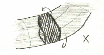
… and then to get rid of the rest of it, we have to wrap around the other way:

(Note: this picture obviously still has a boundary; in order to make it disappear we have to keep wrapping the chain around the torus. In the end, the two boundaries will meet up, at which point they cease to be boundaries at all, and the chain is the entire torus, which is what we were expecting.)
Now, is this $2$-cycle a boundary? Remember that this means it would be a $2$-boundary, or in other words the boundary of a $3$-chain. But a moment’s consideration makes us realize that it could not possibly be the boundary of a $3$-chain: the space is itself only two-dimensional! There’s not enough room to fit a $3$-dimensional shape into it.
——
Dimensional Downstep
Having handled the $2$-dimensional case, we now move to the harder task of classifying $1$-cycles. We will not be so lucky to just be able to count cycles this time: there is lots of room for us to put loops into the space.
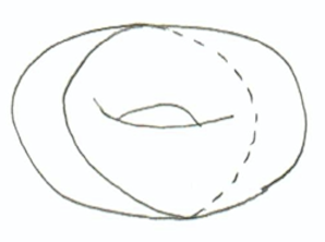
It’s hard to explain, but hard to unsee, that a $1$-cycle is going to be a $1$-boundary unless it “wraps around” the torus somehow: this makes sense with our intuitive definition because it seems like there is a hole in the center:

(In this drawing it kind of looks like you could find a $2$-chain that $\alpha$ is the boundary of. But the dashed part of $\alpha$ is on the back of the torus: if you try to “fill in” the shape you end up on the wrong side of the space.)
In that diagram, you can actually already see another $1$-cycle: all of the grid-lines are 1-cycles! It’s easy to see that the parallel ones are all homologous to each other (take the “rectangle” in between them). It’s less obvious is that none of the “long” ones are homologous to the thickly-drawn $1$-cycle, but this is also true.
We can also see this geometrically, although it is even trickier: notice that $\alpha$ has only one point of intersection with any grid line $\beta$. This poses a problem if we try to find a $2$-chain with boundary $\alpha-\beta$ (which, remember, is also $\alpha+\beta$), because it ends up needing to fill the whole torus:

But we already know that the torus is a $2$-cycle, hence boundaryless, so it couldn’t possibly be that the boundary is $\alpha+\beta$. Therefore, $\alpha$ and $\beta$ cannot be homologous cycles.
——
The One that Got Away
It is natural, at this point, to believe we are done (except that we haven’t mentioned the cycles which are boundaries— now we have). But if we do the calculation for the number of holes, we find that there is an issue. We have $\alpha$ is in a different homology class from $\beta$, and so we’ve found that there are $3$ homology classes (including the class of boundaries). This is a big problem, because $3$ is NOT a power of $2$: It isn’t $2$, and it isn’t $4$ either! We must have missed a cycle.
Indeed we have: I will spare you the trouble of finding it yourself.
But this “missing cycle” raises a more serious concern. How do we know we didn’t miss anything else? Are we absolutely sure there aren’t secretly some more classes hiding around somewhere?
It would surely be impossible to go around checking every single loop: What if you wrap around the center hole four times and then cross the gridline? What if you do the third cycle, but don’t quite close, and then wrap around the center hole and then do the third loop again and then…?
I’m sure that it would be possible to come up with a visual argument like the one I gave above, but you would have to be extremely clever to find it (I do not know one, myself). The point is that when we look at any space that’s even a little bit complicated, it’s not so easy to know when you’re done.
It turns out that there is a method for knowing when to stop counting as well. Unfortunately, that method is quite technical, and this technicality seems to be unavoidable. Actually, the main reason that I delayed writing this sequence so long is because I was trying to find an intuitive way to describe this method; I have not been able to do so. Taking the time right now to build up the required machinery would more than double the length of this sequence, so I am not going to do that. (I am strongly considering writing another sequence, although there is not too much time left >.<)
The final post is a more of an epilogue, which will talk about the highlights from the story of homology’s hotshot cousin: cohomology.
For almost two years, I’ve been skating by, saying “I don’t want to explain homology right now, homology is complicated, ask me later.”.
Later has come, folks. This is the fifth post of a seven-part sequence dedicated to shining light on this beautiful, mysterious beast. (1234567). This is a very important post for us, since we have built up all the background and we will finally see how to use homology to determine the number of holes in a space!
——
Recall that in the last post we gave an algebro-geometric justification which permitted us to understand these two cycles as “essentially the same”:
We thought this was a good thing because both $A$ and $B$ “surround the same hole”, and we only want to count each hole once.
Motivated by this argument, we make the following definitions. If the difference* $A-B$, between two cycles $A$ and $B$, is a boundary, we say that the cycles are homologous, or in other words that they are of the same homology class. This allows us to define the homology of a space as the collection of all homology classes.
Since cycles of different dimensions look qualitatively different, and so they probably surround different-looking holes, it’s natural to want to split up the homology by dimension. We say that the collection of homology classes having dimension $d$ is the $\mathbf{d}^\textbf{th}$ homology group, and is usually written $H_d(X)$, where $X$ is the space in which the chains live.
[ There’s a technicality here: how do we define the dimension of a homology class? After all, homology classes aren’t curves or surfaces or anything; they’re these giant unwieldy collections of many, many chains. However, this “issue” turns out not to be, because any two homologous chains have the same dimension. (This is not totally obvious; it’s worth the effort to draw a picture or two to convince yourself.) Because of this, we can define the dimension of a homology class by determining the dimension of a cycle of that class: any choice will give the same number. ]
[ * You may wonder why I said “difference” instead of “combination”, since $A+B$ and $A-B$ are the same thing, after all, and the former is more geometrically intuitive. The answer is that the subtraction definition works even outside of characteristic $2$; the addition definition does not. ]
——
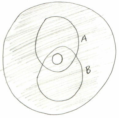
However, even restricting our attention to a single homology group, we’re still not counting holes quite yet! The number of $d$-dimensional holes in the space is actually not the number of $d$-dimensional homology classes. For instance, when $d=1$, we can use a slight variant on our example space: instead of a disk with one hole, take a disk with two holes. See if you can convince yourself that no two of these four loops are homologous.
[ You may be concerned with the innermost square loop: this is the class containing the boundaries. We include it for the same reason we include zero as a number: it’s true that boundaries count for nothing, but nothingness, itself, counts for something. We make this convention for convenience, because it makes the theory nicer (like, way nicer, you’d actually be amazed); this is exactly the same reason that we consider zero to be a number. ]
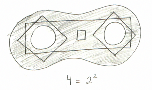
You can keep playing this game: if there are three holes, the picture looks like the one below. (Despite my best efforts, this picture kept turning out a mess; this one I think is at least somewhat legible):
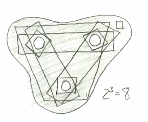
So it turns out that, if you include the class containing all boundaries, the number of classes in a homology group is always a power of $2$; if that number is $2^h$, then we might say that the space has $h$ holes of the corresponding dimension.
By the way: If you think the $2$ in $2^h$ has something to do with being in characteristic $2$, you’re right! But there is also another way to explain it, which perhaps lines up more reasonably with the picture.
People with more advanced mathematics backgrounds may know that $2^h$ is the number of elements in the power set of a set of size $h$, or in other words, is the number of subsets. Applying this knowledge to the situation at hand, it stands to reason that a homology class consists of loops which surround a particular collection of holes. If you believe that the chains I’ve chosen for the pictures above represent “typical” members of their homology classes, then this probably makes sense :) For instance, the fourth cycle in the two-holed space represents the collection “both holes”, and the little squares in both spaces represent the “empty collection” of holes.
——
We’ve made it!
We have described holes, things which “aren’t there”, with genuinely intrinsic features of the space. This was no small feat, and it is worth celebrating.
If this is all you know about homology, you’re in a pretty good place (at least as far as not-being-freaked-out-when-it-gets-mentioned goes). However, we may wish to see some more interesting examples. In the next post, we will grant that wish by peering into some higher-dimensional holes.