Now that it’s no longer possible to experience OTAM as a “dose a day” math fix, I figured I’d try to get around to making a somewhat more accessible organizational scheme. This post is obviously something of a hack, but it was good enough for printed books for hundreds of years it can be good enough for little old OTAM. I’ve split post this into two parts:
First comes a list of significant tags. This means reasonably small collections of posts but contain a high density of the most interesting posts.
And second, underneath a readmore, comes a list of posts (or drafted posts) which are significant in their own right but cannot be easily found from the tags. [The eight posts in this list marked with stars and italics are, in my opinion, the absolute highlights of this blog.]
1000 (Day 1000) [literally first day I was caught up since Jan2015 >.< ]
Top Contributors:
Posts dedicated to the work/talks of Theo: 1234567891011
Posts dedicated to the work/talks of Vic Reiner: 12345678910
Posts dedicated to the talks of Laura Escobar: 12345678910
It looks you three lead the pack by a longshot; I had some ideas but ultimately I couldn’t find anyone doing better than Maria Gillespie who has 12345 with the last two being a little bit iffy. But if you don’t count that then it looks like it’s just lots of people tied at three posts
This talk was given by Elizabeth Kelley at our student combinatorics seminar. She cited Godbole, Kurtz, Pralat, and Zhang as collaborators. One of these (Pralat, I think) was originally an editor, but then made substantial contributions to the project. This post is intended to be elementary.
[ Personal note: This is the last talk post I will be writing for OTAM. It seems fitting, since Elizabeth and I went to the same undergrad; I have actually known her for almost as long as I have been doing mathematics. ]
It did begin with this: Let $G$ be a graph with a vertex-weighting (i.e. an assignment of nonnegative reals to each vertex). An acquisition move is a “complete transfer of weight” from a low-weight vertex to an adjacent higher-weight vertex. In other words, if the weights before the move are $w\leq x$, then the weights after the move are $0\leq w+x$ (respectively).
[ For the sake of not cluttering up the definitions with trivialities, we will say that both of the weights involved in an acquisition move must be strictly positive— that is: not zero. ]
From this, a bunch of definitions follow in quick succession.
A sequence of acquisition moves is called an acquisition protocol if it is maximal, i.e. after performing all of the moves, no further move is possible.
The set of nonzero-weight vertices after performing an acquisition protocol is called a residual set.
Finally, the acquisition number of $G$ is the minimum size of any residual set. We write it as $a(G)$.
This explains half of the title. The other half of the title, is perhaps a bit more self-explanatory. A lot is known about acquisition numbers when, say, all vertices are given weight $1$. Less is known in other contexts, but the goal of this paper is to ask what we “should” expect for paths. More precisely: if we give the vertices random weights, what is the expected acquisition number?
——
Fekete’s Lemma
A sequence of real numbers $(x_n)$ is called subadditive if it does what the name suggests: for all $n$ and $m$
$$ x_{n+m} \leq x_n + x_m.$$
This is a pretty general construction, and tons of sequences do this: certainly any decreasing sequence will, and also most reasonable sequences that grow slower than linear ($\log(n)$ works, for instance). Usually, when the situation is so general, it is hard to say anything at all about them, but in this case things are different:
Lemma (Fekete). Given any subadditive sequence $(x_n)$, the limit of $x_n/n$ exists, and moreover
(This lemma has one of my favorite proofs, which is essentially the same as the one given in this NOTSB post; just reverse all the inequalities and repeat the argument with liminf/limsup replaced by lim/inf.)
This means that whenever you have a subadditive sequence, it makes sense to ask about its growth rate, which is just the limit that Fekete guarantees exists. Less formally, it is the number $c$ such that $x_n \approx cn$ as $n$ gets large. (Perhaps in this formulation is the existence statement so striking: why should there be such a number at all? But Fekete states that there is.)
As it happens, it is pretty easy to prove that $a(P_n)$, where the path $P_n$ on $n$ vertices has been weighted with all 1s, forms a subadditive sequence.
This proof doesn’t use much about the weightings at all: it requires only that they are “consistent” in some technical sense. The punchline for our purposes is that $a(P_n)$ continues to form a subadditive sequence when the paths are weighted by independent identically distributed random variables.
——
Numbers, Please!
In the paper, Kelley considered the case when the vertex weights were distributed as a Poisson distribution. This is a thing whose details aren’t too important, but if you’re familiar with it you may be wondering why this instead of anything else? The answer is because when you know the answer for the Poisson model, you also know it in a more physically reasonable model: you start with a fixed amount of weight and you distribute it randomly to the vertices.
[ The process by which you use Poisson to understand the latter model is called “dePoissonization”, which makes me smile: to me it brings to mind images of someone hunched over their counter trying to scrub the fish smell out of it. ]
But enough justification: what’s the answer? Well, we don’t actually know the number on the nose, but here’s a good first step:
Theorem (Godbole–Kelley–Kurtz–Pralat–Zhang). Let the vertices of $P_n$ be weighted by Poisson random variables of mean $1$. Then $0.242n \leq \Bbb E[a(P_n)] \leq 0.375n$.
The proof of this theorem is mostly number-crunching, except for one crucial insight for each inequality: This step is easier to prove for the lower bound: after we have assigned numbers for the random variables, check which functions have been given the weight zero and look at the “islands” between them. Acquisition moves cannot make these islands interact, and so we can deal with them separately, so $\Bbb E[a(P_n)]$ splits up into a sum of smaller expectations based on the size of the islands. In a strong sense “most” of the islands will be small, and so you get a pretty good approximation just by calculating the first couple terms.
To get an upper bound, you need to think of strategies which will work no matter low long the path is and what variables are used. The most naïve strategy is to just pair off vertices of the path and send the smaller one in the pair to the larger one. This may or may not be an acquisition protocol, but you will always cut the residual set size (roughly) in half. Following even this naïve strategy is good enough to give the 0.375.
Both of these steps are fairly conceptually straightforward, but it becomes very difficult to calculate all the possibilities as you get further into the sum; in other words, it’s a perfect problem for looking to computer assistance. This allows us to get theoretical bounds $0.29523n \leq \Bbb E[a(P_n)] \leq 0.29576n$; and of course it would not be hard to get better results by computing more terms, but at some point it’s wiser to start looking for sharper theoretical tools rather than just trying to throw more computing power toward increasingly minuscule improvements.
This talk was given by Jay Yang as a joint talk for this year’s CA+ conference and our usual weekly combinatorics seminar. He cited Daniel Erman as a collaborator.
——
Ein–Lazarsfeld Behavior
Yang began the talk with a fairly dense question: what is the asymptotic behavior of a Betti table? He then spent about 20 minutes doing some unpacking.
What is a Betti table? This has an “easy” answer, which is that it is an infinite matrix of numbers $\beta_{ij}$ defined as $\dim \text{Tor}^i(M)_j$, but this is maybe not the most readable thing if you’re not very well-versed in derived functors. Fortunately, exactly what the Betti table is is not super important for understanding the narrative of the talk.
But, for the sake of completeness we briefly give a quote-unquote elementary description: Given a module $M$, produce its minimal free resolution— that is, an exact sequence $\cdots\to F_2\to F_1\to F_0\to M\to 0$, where $F_i$ are all free, and the maps, interpreted as matrices, contain no constant terms. If $M$ is a graded module over a graded ring, then the $F_i$ are also graded, and so we can ask for a basis for the submodule of (homogeneous) elements of degree $j$. This number is the Betti table entry $\beta_{i,j}$.
What do we mean by asymptotic? We need to have something going off to infinity, clearly, but exactly what? There are several ways to answer this question: one which Yang did not explore was the idea of embedding by degree-$n$ line bundles, and sending $n\to\infty$. Instead of doing that, we will force our modules $M$ to come from random graphs, and then take asymptotic to mean sending the number of vertices to infinity.
What do we mean by behavior? Again, Yang deviates from the usual path: the most well-studied kind of long-term behavior is the “$N_p$” question “For how long is the resolution linear?” But instead of doing this, we will discuss the sorts of behaviors which were analyzed by Ein and Lazarsfeld.
One of these behaviors, which he spent most of the time talking about, concerns the support of the table, and stems from their 2012 result:
Theorem (Ein–Lazarsfeld). If $X$ is a $d$-dimensional smooth projective variety, and $A$ a very-ample divisor, then
$$ \lim_{n\to\infty} \frac{ \# \text{nonzero entries of the } k^\text{th} \text{ row of } X_n}{\text{projdim}(X_n) + 1} = 1$$
where $X_n$ is the homogeneous coordinate ring of $X$ embedded by $nA$, and $1\leq k\leq d$.
The same limit formula was reached in 2014 and 2016 for different classes of rings than $X_n$.
Ein and Lazarsfeld also showed another kind of asymptotic behavior together with Erman in a similar situation: namely, that the function $f_n$ sending $i$ to a Betti table element $\beta_{i,i+1}(S_n/I_n)$ converges to a binomial distribution (after appropriate normalization).
Yang examined both of these behaviors to see if they could be replicated in a different context: that of random flag complexes.
——
Random Flag Complexes
Arandom graph is, techncially speaking, any random variable whose output is a graph. But most of the time when people talk about random graphs, they mean the Erdős–Rényi model of a random graph, denoted $G(n,p)$:
Any graph consists of vertices and edges. So pick how many vertices you want ($n$), and then pick a number $0\leq p\leq 1$ which represents the probability that any particular edge is in the graph. Then take the complete graph on $n$ vertices, assign independent uniform random variables, and remove each edge whose output is larger than $p$.
This gives rise to the notion of an Erdős–Rényi random flag complex, denoted $\Delta(n,p)$, by taking a $G(n,p)$ and then constructing its flag complex:
And finally, we can describe a Erdős–Rényi random monomial ideal, denoted $I(n,p)$ by taking a $\Delta(n,p)$ and then constructing its Stanley-Reisner ideal.
The punchlines is that $I(n,p)$ will, in nice cases, exhibit the Ein-Lazarsfeld behaviors:
Theorem (Erman–Yang). Fix $r>1$ and $F$ a field. Then for $1\leq k\leq r+1$ and $n^{-1/r} \ll p \ll 1$, we have
$$ \lim_{n\to\infty} \frac{ \# \text{nonzero entries of the } k^\text{th} \text{ row of } F[x_1,\dots, x_n]/I(n,p)}{\text{projdim}(F[x_1,\dots, x_n]/I(n,p)) + 1} = 1,$$
where the limit is taken in probability
Theorem (Erman–Yang). For $0<c<1$ and $F$ a field, the function sequence $(f_n)$ defined by
$$ f_n(i) = \Bbb E \Big[\beta_{i,i+1}(F[x_1,\dots, x_n]/I(n,p)\Big]$$ converges to a binomial distribution (after appropriate normalization).
The latter statement can be made considerably stronger, eliminating expected values in exchange for requiring convergence in probability. But he stated it in this generality so that he could concluded the talk by giving proof sketches for both statements (which I won’t reproduce here).
So I don’t really remember why I was thinking about this but it’s flooding back and I’m going to forget it in an hour so I have to write it now.
——
My major advisor (not my thesis advisor) in undergrad was a fellow named Michael Orrison. He spends his time thinking about representation theory and algebraic statistics. It’s pretty cool stuff.
During my four years in college, I’ve took three courses from him. One was Discrete, a sort of intro-to-proofs course, and I am relatively confident in saying that it was my favorite course I will ever take in my life*. One was Algebra I, which was… challenging.
[ * although, I have to admit, 9th grade history does come pretty close. ]
The last was a special topics course about harmonic analysis on finite groups, which is a stone’s throw from his research. In that class I learned three things. I learned that there is a difference between being good at presentations and being good at lectures. I learned why combinatorialists care about representation theory. And I also learned this:
At some point in the last third of the course, he takes a break from lecturing to get all starry-eyed. His #passion has been out in full force during this lecture. He’s reached a conclusion, and he turns to the class and tells us about his journey into this field. I couldn’t recount it; I don’t remember any of it. I do remember that he conceptualized the work in his discipline as a story, a story that he and his colleagues were privileged to be allowed to read.
In passing, in transition to a more important thing, he said “I’ve been thinking about this story now for 20 years, and…”. And somehow, at that moment, the incredible enormity of that statement resonated with me.
I think of myself as a pretty committed individual. I have projects that my parents started in grade school under my name and I still now actually run them. I played piano from kindergarden to graduation. I spent long enough drawing cartoons in a forum that they let me moderate it. I’m writing a blog where I’m trying to write 1000 posts about math 1000 days (it’s pretty cool you should check it out). And yet—
20 years.
I was not quite 21 years old at the time. 20 years isn’t a length of time that I have been “doing” anything. 20 years is a length of time that I have been “existing”. The idea of doingsomething for 20 years, is, still, mind-numbing. Literally. My brain shuts down as it tries to imagine.
How old are you?
What fraction of your life is 20 years?
(Someone will read this who wasn’t alive 20 years ago. Someone will read this whose parents didn’t know each other 20 years ago.)
Orrison has been thinking about that story since I was pooping in diapers. Every single moment of embarrassment or irritation, every time I ran away from home, every stupid game I got obsessed with, every argument with a friend, my whole damn creative life (and longer) was spent thinking about this story.
And it occurs to me: the fact that I find this inspiring (instead of, you know: deeply, existentially terrifying) is one of the best indications I’ve ever had that I would be in the math game for the long haul.
This talk was given by Lauren Williams at this year’s CA+ conference. She cited Reitsch has her collaborator. (It was not the winner of this conference; I had to miss the winning talk, unfortunately.)
Her talk was pretty fast, and in the end there was still more to talk about than she had time for. In particular, she frequently alluded to the cluster algebra stuff going on in the background but we never explicitly talked about it. Also, she explicitly said that she wanted to “downplay” the mirror symmetry. My impression from this, and what snippets I’ve gotten from other people, is that mirror symmetry seems to be very hard to explain in a convincing way.
In any case, she spent the first half of the talk laying out a detailed outline, without defining too much. This post will pretty much follow that outline exclusively; leaving out the more detailed explicit combinatorial constructions involving plabic graphs. In particular, this means I’ll be skipping a lot of definitions, so this post will not be elementary.
——
NObodies
The surviving words in the title are Newton–Okounkov bodies and Grassmannians. The latter is fairly easy to describe if you feel good about linear stuff: the Grassmannian $\text{Gr_d}(\Bbb C^n)$ is the collection of all $d$-dimensional subspaces of the vector space $\Bbb C^n$.
[ Of course there is a lot more that one can say about the Grassmannian, but that won’t be necessary here. ]
TheNewton-Okounkov body is one of those combinatorial constructions that I said I was going to leave out, but let me try to give some general flavor. Given a toric variety, we can construct a thing called the “moment polytope”; this turns out to be pretty darn useful for understanding toric varieties. The Newton-Okounkov body $\Delta$ (or NObody) is an object defined in an attempt to produce similarly nice geometric objects for arbitrary varieties.
[ NObodies, in particular, need not be polytopes, in which case a lot of the good combinatorics from moment polytopes isn’t accessible. But all of the NObodies associated to Grassmannians turn out to be polytopes, and so the dream is still alive. ]
So if we are going to want to talk about NObodies, there had better be some varieties hanging around. These varieties are the images of a map $(\Bbb C^\times)^N \to \text{Gr}_{n-k}(\Bbb C^n)$ which is defined with the help of a particular kind of plabic graph. We’ll denote the NObody of such a thing by $\Delta_G$, where $G$ is the corresponding plabic graph.
The lattice points of $\Delta_G$ tell us something about the geometry of the relevant Grassmanian. More specifically, if we scale $\Delta_G$ by a factor of $r$, the integer lattice points of $r\Delta_G$ turn out to define a basis for the space of sections $H^0(X,\mathcal O(rD))$, where $D$ is the ample divisor $\{P_{1,2,\dots, n-k}=0\}$.
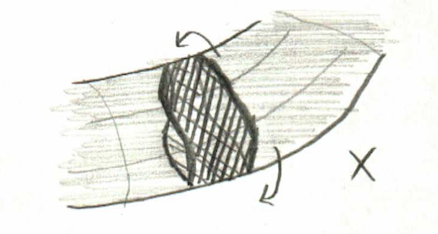
All of this lives on the “A model” side of the mirror symmetry construction. On the other side of the mirror, something different happens.
——
Bee Model
The A model gets all of its power from the Grassmannian, and there is an analogous shape that governs everything in the B model as well. This shape isn’t much harder to describe, but it is a little more technical: it is the subset of $\text{Gr}_k(\Bbb C^n)$ containing those subspaces for which every cyclic Plücker coordinate is nonzero. And a cyclic Plücker coordinate is the determinant of every $k\times k$ submatrix containing columns $i+1, i+2,\dots, i+k$, where the $(n+1)^\text{th}$ row is the first row, and so on).
Because of an even shorter and more technical way to describe this shape (the complement of the anticanonical divisor) there exists a function mapping it to $\Bbb C(x)$ called the superpotential, which she very intentionally said nothing about. I’ve written briefly about something called a “superpotential” as part of one of the combinatorics seminar talks. This had the advantage that we actually defined the darn thing, but still the same problem that we don’t really know what this thing is for. It must be one of those things where it’s not so easy to say.
Analogous to $\Phi_G$ in the A model is a different map called the cluster chart $\Psi_G$, also defined by a plabic graph $G$. This defines coordinates on the B model shape, and so we can try to write the superpotential in terms of those coordinates. If you do this, you get a polynomial map, and if you tropicalize that map, the resulting graph is a polytope. We denote that polytope by $Q_G$.
——
The Miracle
Those of you who have done enough mathematics (even if it doesn’t have anything to do with this stuff), probably know what’s coming next:
Theorem (Reitsch–Williams, 2015). For a fixed plabic graph $G$,
$$ \Delta_G = Q_G. $$
The fact that $\Delta_G$ and $Q_G$ are related at all is not obvious. The constructions are very different from one another: one comes from a NObody associated to walks on the plabic graph, and the other comes from a tropicalization of the superpotential.
But what is even more amazing is that they’re not just related: they are equal. And Williams said this in no uncertain terms: equal means equal. Like, as sets. No combinatorial equivalence, or rescaling, or isometry, or anything. And I dunno about you, but I find that pretty miraculous.
This talk was given by Alex Yong at this year’s CA+ conference. He cited Robichaux as a collaborator, as well as high school student Anshul Adve.
——
Factorial Schur Functions
As with all the best combinatorics, we start with a game.
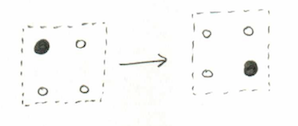
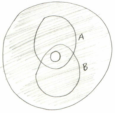
Given a partition (possibly with some zero parts), draw its Young diagram but replace the boxes with black dots and the “positions without boxes” with white dots. Don’t have any extra rows, but extra columns are okay. For instance, the partition $(2,2,0)$ corresponds to this picture
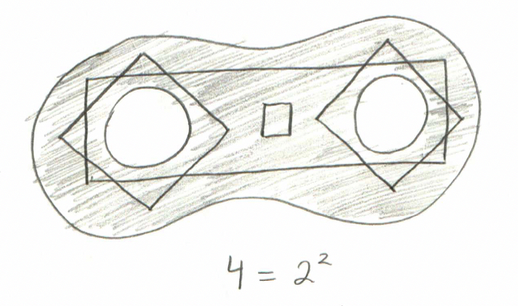
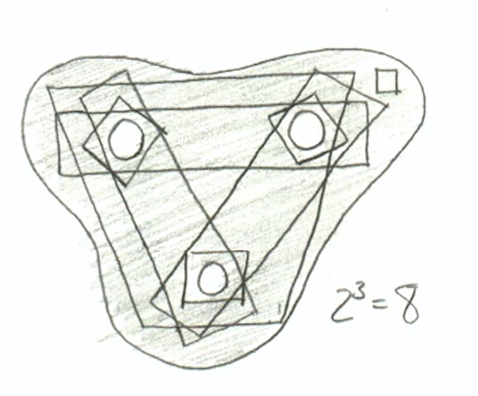
We then make moves according to the following rule, anytime we see a black dot in a TL corner of a square that’s otherwise white, we can move it to the BR corner:
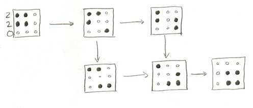
We make this move wherever possible until there are no more available. The set of all diagrams that can be obtained this way, starting with the partition $\lambda$ will be called, uncreatively, $\text{Black}(\lambda)$. To keep with our example, here is $\text{Black}((2,2,0))$:
Now it is time for some algebra: we are going to describe a polynomial in two sets of variables $X=x_1,\dots, x_r$, where $r$ is the number of rows; and $Y=y_1, y_2, y_3,\dots$ representing the columns. First, we define the weight of a diagram $\text{wt}(D)$ to be the product of every $x_i-y_j$, for all $i$ and $j$ such that there is a black dot in row $i$ and column $j$.
Finally, define the factorial Schur function $s_\lambda(X,Y)$ to be the sum of $\text{wt}(D)$ over all diagrams $D\in\text{Black}(\lambda)$. As a formula:
$$ s_\lambda(X,Y) = \sum_{D\in\text{Black}(\lambda)} ~~ \prod_{(i,j)\text{ is black}} x_i-y_j. $$
——
Littlewood-Richardson Polynomials
The reason that factorial Schur functions are called that is because if you plug $y_i=0$ for every $y$, the resulting polynomial is really, honestly, the Schur polynomial. Schur functions form a basis for the symmetric algebra, and so we might hope that the symmetric Schur functions are the basis for something. This hope turns out to be validated: it is a $\Bbb Z[Y]$-module basis of $\Lambda_n\otimes \Bbb Z[Y]$ (The last symbol there is polynomial algebra in the $y$-variables, and the symbol in the middle is a tensor product)
Because of that, this means that $s_\lambda(X,Y)s_\mu(X,Y)$ must be some linear combination, and so we can ask for the structure coefficients $C_{\lambda,\mu}^\nu(Y)$. We write the $Y$ there because in general these things can be an element in $\Bbb Z[Y]$; in other words, can be a polynomial in the $y$-variables.
Since they specialize to the Littlewood-Richardson coefficients when $y_i=0$, we call these $C_{\lambda,\mu}^\nu$ the Littlewood-Richardson Polynomials
[ Because of the geometric interpretation of ordinary Littlewood-Richardson coefficients, we know that they are nonnegative integers; you may ask whether the LR-polynomials are also positive (in that all the coefficients are negative). The answer is no, but they are positive as polynomials in $z_i:=y_{i+1}-y_i$. ]
——
Polynomial Time
In 2005, one day after the other, two papers were posted to the arXiv, both claiming to have proven the following theorem:
Theorem (DeLoera–McAllister 2006, Mulmuley–Narayanan–Sohoni 2012*). There is an algorithm for determining whether or not the Littlewood-Richardson coefficient $c_{\lambda,\mu}^\nu=0$ in polynomial time.
If you’re not super familiar with “polynomial time”, feel free to substitute the word “quickly” anywhere you see it; this isn’t necessarily true but it’s a respectable approximation.
This naturally raises the question of whether the Littlewood-Richardson polynomials can also be determined to be zero or not in polynomial time. As the title of the talk suggests— and as Adve, Robichaux, and Yong proved— the answer is yes. The rest of this section is devoted to a proof sketch.
There is a celebrated proof due to Knutson–Tao which proves the so-called saturation conjecture, that $c_{\lambda,\mu}^\nu=0$ if and only if $c_{N\lambda,N\mu}^{N\nu}=0$ for all $N$. At this point, Yong talked a little bit about the history of that conjecture:
In the 19th century, people were asking this question about Hermetian matrices.
In 1962 Horn conjectured a bunch of inequalities which resolved the question.
In 1994 Klyachko solved the problem, but didn’t use Horn’s inequalities.
Soon after, it was realized that the saturation conjecture was sufficient to prove Horn’s inequalities.
In 1998, Knutson and Tao published their proof.
The argument they made in this paper was refined by a 2013 theorem of a different ARY team: Anderson, Richmond, and Yong. They showed that the analogous statement is true for the Littlewood–Richardson polynomials: $C_{\lambda,\mu}^\nu(Y)=0$ if and only if $C_{N\lambda,N\mu}^{N\nu}(Y)=0$ for all $N$.
The major innovation made by the new ARY team (Adve, Robichaux, and Yong) constructed a family of polytopes $P_{\lambda,\mu}^\nu$ with the following properties:
scaling the polytope by a factor of $N$ is the same as scaling the partitions by a factor of N, i.e. $P_{N\lambda,N\mu}^{N\nu} = NP_{\lambda,\mu}^\nu$,
and the crucial bit: $P_{\lambda,\mu}^\nu$ has an integer lattice point if and only if $C_{\lambda,\mu}^{\nu}(Y)\neq 0$
In particular, this implies that the “polynomial saturation conjecture” can be used to reduce the question of $C_{\lambda,\mu}^{\nu}(Y)\neq 0$ to figuring out whether $P_{\lambda,\mu}^\nu$ is the empty polytope. And this, finally, is a problem which is known to be solvable in polynomial time, which concludes the proof.
——
[ * The dates listed above are the publication dates of the papers that the two teams wrote. “So that tells you something about publishing in mathematics”, Yong says. Perhaps, but… I’m not sure what. I’m assuming that what he was getting at is this: The names in the latter team are nothing to scoff at, by a long shot; I mean, I have heard all five of these names before in other contexts. But the prestige associated to the names in the former team might have made that paper subject to less scrutiny than the latter. Or perhaps he just meant that the capricious turns of fate can turn what “should be” a short procedure into a long one. ]
After reviewing past tests from both my university and others, I’ve determined that written qualifying exams in mathematics graduate programs are like the math subject GRE on crack.
For the math subject GRE (note: not the math portion of the general GRE), the best way to prepare is:
1) Read the Princeton review book to remember how to do calculus, differential equations, and linear algebra.
2) Do problems until your eyes bleed, then do some more (including taking all of the available practice tests).
This worked very well for me. There’s no time to think on the test if you want to answer all the questions – everything needs to be automatic, you need to be able to solve every problem on sight.
My approach to my upcoming qualifying exam has been basically the same, expect step 1 is has been replaced by “review everything on the syllabus.” Most of which I purportedly know, but have forgotten. I have yet to start step 2, but hope to get there soon.
Some thoughts:
Many of the problems that appear on these exams are (like the GRE, like the SAT, etc) variations on well-known themes. For example, if your exam covers complex analysis, there will always be an integral you need to do by residues. Always. And if your exam covers algebra, you will almost always need to compute a Galois group. There are less obvious examples, too. I’ve seen the example from Dummit and Foote about counting monic irreducible polynomials of a fixed degree a few times, for instance.
The best way to identify these is probably to mass-solve past exams and note the patterns. But generally, I’m making it my goal to know every to do everything on these lists (see here for the complex analysis list, for example).
Knowing about messy proofs of hard theorems seems basically pointless. For example, no qualifying exam asks about proving the fundamental theorem of Galois theory, or the homotopy version of Cauchy’s theorem, etc. You DO need to know how to prove the simple stuff, but these are classic and you can see them coming a mile away – a finite multiplicative subgroup of a field is cyclic, Liouville’s theorem, the fundamental theorem of algebra, etc.
Once you solve enough problems, a lot of the test questions you can see how to solve immediately (e.g. “Oh, right, this integral needs to be done by residues”) which allows you to save time for the trickier ones. Like the math GRE, you definitely do NOT want to spend time thinking about every question. You’ll run out of time, get stuck, etc.
I was under the impression that qualifying exams were more proof oriented, whereas I always got the sense that the math GRE was based on knowing which quick computational trick you had to do. So I mean, finding a Galois group is something you’d definitely never see on the GRE but it does seem more rote than I’d expect (rote is a bit too nice of a word here, I know finding a Galois group could be tough)
So am I mistaken? I haven’t taken any qualifying exams yet.
If you ever come back to the world of tumblr, @ryanandmath, I’d like to hear what your thoughts are, since I’d guess you’ve taken a qualifying exam or two by now :)
In absence of that, I’ll say that I had similar thoughts to you when I started grad school, including when I was studying for the real analysis exam. But nowadays I do mostly agree with OP: my written quals were pretty darn “memorize-able”.
In particular, I offer this anecdotal evidence: I think the exam where I went in with the worst preparation was algebra (either for the subject matter or for the exam), and that was also the only one where I felt that I might have been able to finish if I’d had another hour.
On the other hand, I was way more prepared for topology, from the taking-an-exam point of view, than I was for real analysis. But I had a lot more background in real analysis than I had in topology, and consequentially I found the test easier.** I guess I just bring this up to say that— despite the similarities— I found the written quals not as easily gameable, nor as amenable to “do problems until your eyes bleed” quasi-cramming, as was the GRE subject test.
——
I don’t want to generalize too quickly: I know that UMN was in the process of trying to make its written quals a little more predictable— except that now there is one guy responsible for writing three of the four exams and it’s clear that he doesn’t buy into this idea as the people he took over from.
For the differential side of topology, which I have never really learned to my satisfaction (despite my attempts*), this predictable structure really paid off for me: in particular, I was pretty darn sure there would be a question about computing Lie brackets, and there would be one asking me whether a given form was exact, and so on.
I also know that UMN doesn’t use the written quals as a weed-out mechanism, which is not universally true. If anything can be said to be that, it would be the oral quals instead, but that is a completely different style of exam.
——
* Actually, the phenomenon I’m describing can maybe be seen clearly just by going through my writeups in that tag. You can see pretty clearly when a new guy started writing, but within the two “blocks”, everything is pretty consistent.
** My studying for the real analysis exam (which, however, I had considerable background in) was less about solving problems and more about just looking over the old exams and seeing what the “usual tricks” were.
For instance, most Prove/Disprove real analysis questions
about sets with weird measure properties, could be reliably tested against the fat Cantor set or a set containing every rational with nonzero-measure complement
about Hilbert spaces, would reliably benefit from using
Most inequalities needed to use Hölder, most “evaluate this series” questions were really about Parseval’s theorem, and there was always a question testing the hypotheses of Fubini’s theorem.
But last spring the new guy was writing real analysis and so… yeah that strategy wouldn’t have worked very well at all. So: a vague idea of departmental politics + who wrote which exams and when; these are not bad ideas for contextualizing what you’re studying.
This talk was given by Claudia Polini at the 2017 CA+ conference. This post will not attempt to be elementary.
——
Rees Rings
The scope of the talk was ostensibly rather modest: “There is very little that we can say in general [about Rees rings]. This talk is about what can be said in some general situations.”
The sorts of “things” that we were trying to talk about was to determine when a certain ideal is of “fibre type”; to explain what this means and why we care about it requires rather more setup.
Let $k$ be a field and $R=k[x_1,\dots, x_d]$ be a polynomial ring. Given a bunch of homogeneous polynomials $f_1,\dots, f_n$ of degree $\delta$, consider the map $f=[f_1 : \dots : f_n]$ sending $k\Bbb P^{n-1}$ to $k\Bbb P^{n-1}$. Let the coordinate ring of the image— i.e. the collection of all polynomial functions on the image— be denoted $A(X)$. This ring fits into a short exact sequence
$$ 0 \to I(X) \to k[y] \to A(X) \to 0 $$
for some $k$-algebra $I(X)$.
The story so far is very biased in favor of the image. But we may gain more information by looking at, instead of $A(X)$, the following analogous setup: let $I=(f_1,\dots, f_n)$ be the ideal that these X generate, and define the Rees ring $\mathcal R(I)$ to be $R[It]$. The Rees ring also fits into a short exact sequence
$$ 0 \to J \to k[x,y] \to \mathcal R(I) \to 0. $$
One can naturally identity $I(X)\subset J$, and the question is: if you know $I(X)$, can you determine $J$. And the answer is no, but you can if the ideal $I$ has fibre type.
——
Ideals of Fibre Type
The Rees ring also fits into a different short exact sequence, as a quotient of the symmetric algebra in the $f$s:
This turns out to be very useful, because it gives several equivalent descriptions of what it means to be of fibre type: in particular, $\mathcal A= I(X)\cdot S(I)$, or also that $J$ is generated in degrees $(*,1)$ and $(0,*)$. This notation means that the $x$-degree can be whatever, but if it is not zero then the $y$-degree is forced to be $1$.
At this point, Polini did some technical work on the board that I didn’t follow, but her conclusion was that we were going to assume that $\mathcal A$ is a local cohomology module, namely $\mathcal A = H_{\mathfrak m}^0(\Lambda(I(\delta)))$
[ I believe that the $(\delta)$ notation means to construct an ideal which is the same as a set, but has a different notion of “degree”: all degrees are supposed to be shifted downward by $\delta$. Or perhaps upward… I was never clear what the goal of the degree shifting was supposed to be in this talk. ]
In this case, we have an even more workable characterization of fibre type: $\mathcal A_{\bullet, j}$ is generated in degree $0$ for all $j$.
——
Approximate Resolutions
It turns out that, under the local cohomology assumption we made before, the problem is completely solved if we had a minimal free resolution of the symmetric powers $\text{Sym}_j(I(\delta))$. [ No, I don’t know why. ]
Unfortunately, this will never happen because computing minimal free resolutions of symmetric powers is too hard. So instead we may hope for an approximate resolution. This is where, instead of a complex of free modules, we ask only that the complex contains finitely generated modules; and moreover we make no restrictions whatsoever on the higher homology groups. It’s worth noting, though, that in practice the power of approximate resolutions comes when you can assume some control on the higher homology groups; for instance $H_i(F_\bullet)\leq i$.
In 1979, Weyman published a construction which gives an approximate resolution $(C_{j,\bullet})$ for the $j^\text{th}$ symmetric power of $I(\delta)$, assuming you have a free resolution $(F_\bullet)$ of $I$. The details are not nearly as gory as you might expect:
where the direct sum is taken over all compositions $\alpha=(a_1,\dots, a_k)$ with $\sum a_i = j$ and $\sum ia_i=t$.
In any case, this was the technique which Polini used to prove her result. That states, among other things, that $\mathcal A$ is generated in degrees at most $(d-1)(\text{reg}(I)-\delta)$ under some technical (and not insubstantial) restrictions on the ideal. The details of the conditions are important for the novelty of the work, but ultimately it is this control on the degrees which generated $\mathcal A$ that are the important theoretical advance.
At the end of her talk, she mentioned several other techniques which people are using to try to get bounds on these degrees. These will hopefully allow us to work with other, and perhaps larger, classes of rings.
This is the second of two posts based on a talk given at Dmitriy Bilyk at our probability seminar (the first one is here). I don’t usually go to probability seminar, but have enjoyed Dmitriy’s talks in the past, and I didn’t regret it this time either :)
——
Semirandom Methods
In the previous post we defined the Riesz energy and the discrepancy, and we said that (deterministic!) sets which minimize either of these things should be said to be “uniformly distributed”. We also mentioned that in general, we don’t know very many deterministic methods for creating uniformly distributed points on the sphere.
Using these two measures, the situation does not improve much for purely deterministic methods. But it turns out that there are two semirandom methods that do pretty well by both measures. The easiest to describe, and the most successful, is called jittered sampling: take one point uniformly at random from each part of any “regular equal-area partition”, which is some technical thing that’s not important. What’s important are the results:
It on average achieves the upper bound in Beck’s theorem of $\approx N^{-\frac12-\frac1{2d}}\sqrt{\log N}$.
It doesn’t optimize the Riesz energies, but it “almost” does so, in a way that Bilyk did not describe.
Somewhat more complicated is the determinental point process. It seems that nowadays these are of pretty big interest to machine learning, idk. But I do know (or rather, Bilyk knows and so I can inform you) that it enjoys similar properties to jittered sampling, although it is not quite as good in the discrepancy sense (I believe it’s $\log N$ instead of $\sqrt{\log N}$, but don’t quote me).
He also talked about some work that he did with Feng Dai and my colleague and friend Ryan Matzke related to the Stolarsky Invariance Principle. I think this produces a third semirandom method which has similarly nice properties, although to be honest I did not really follow that part of the talk >.>
However, there has recently been a new theoretical advance which has allowed for the possibility of more deterministic methods; we’ll spend the rest of the post talking abut that.
——
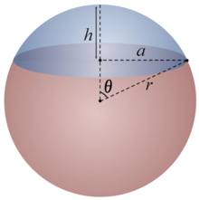
Uniform Tessellations
Given two points $x$ and $y$ on the sphere, and a random hyperplane, the probability that the hyperplane separates them is the spherical distance between them $d(x,y)$ [technicality: on a sphere of appropriate radius such that the distance from the north to the south pole is $1$]. Motivated by this fact, we define a Hamming distance, relative to a given set $Z=\{z_1,\dots, z_N\}$, between two points $x$ and $y$ as
[ Those of you who know a different notion of Hamming distance may be interested in reading Section 1.1 of this paper, which lays out the relationship very clearly. ]
For any fixed $x$ and $y$, as $N\to\infty$, the expected Hamming distance (over all sets of size $N$) converges to $d(x,y)$; this says that the Hamming distance is a fairly reasonable object. But what we actually want to do is the following: for any set $X\subset S^d$ (which need not be finite), we say that $Z$ induces a $\delta$-uniform tessellation of $X$ in the event that $\sup_X |d_Z(x,y)-d(x,y)| \leq \delta$.
The goal is to find small $N$ which admit sets that induce $\delta$-uniform tessellations of $X$; ideally the smallest such $N$. Of course finding large $N$ is not very hard: as the number of hyperplanes grows, there will eventually be some set which does this. Indeed, the existence of $\delta$-uniform tessellations can be understood as “speed of convergence” results for the convergence $d_Z\to d$ mentioned above.
Of course the answer is going to have to depend somehow on the geometry of $X$, and so our answer is going to have to depend on some quantified statement of how “bad” the geometry is. I do not wish to explain exactly how this is done, but Bilyk and Lacey were able to come up with two answers:
Theorem (Bilyk–Lacey). There exist constants $C$ and $C’$ such that it is sufficient for either $N\geq C\delta^{-3}\omega(X)$, or $N\geq C’\delta^{-2}H(X)$.
Here, $\omega(X)$ is a classically studied geometric statistic, and $H(X)$ is a variant which Bilyk and Lacey invented.
This dramatically improves on previous results, and in particular gets us tantalizingly close to the (previously) conjectured optimal lower bound, which is $C\delta^{-2}\omega(X)$. You can see that this conjecture is sort of the combination of their two results: it takes the $-2$ power from the second bound but still uses the $\omega$ statistic. Unfortunately, Bilyk did not seem optimistic that there were many technical improvements that could be made to their idea. So breaking the $-3$ barrier with the $\omega$ is probably still in want of another innovation.
This post is going to try and explain the concepts of Lagrangian mechanics, with minimal derivations and mathematical notation. By the end of it, hopefully you will know what my URL is all about.
Some mechanicses which happened in the past
In 1687, Isaac Newton became the famousest scientist jerk in Europe by writing a book called Philosophiæ Naturalis Principia Mathematica. The book gave a framework of describing motion of objects that worked just as well for stuff in space as objects on the ground. Physicists spent the next couple of hundred years figuring out all the different things it could be applied to.
(Newton’s mechanics eventually got downgraded to ‘merely a very good approximation’ when quantum mechanics and relativity came along to complicate things in the 1900s.)
In 1788, Joseph-Louise Lagrange found a different way to put Newton’s mechanics together, using some mathematical machinery called Calculus of Variations. This turned out to be a very useful way to look at mechanics, almost always much easier to operate, and also, like, the basis for all theoretical physics today.
We call this Lagrangian mechanics.
What’s the point of a mechanics?
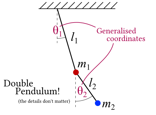
The way we think of it these days is, whatever we’re trying to describe is a physical system. For example, this cool double pendulum.
The physical system has a state - “the pieces of the system are arranged this way”. We can describe the state with a list of numbers. The double pendulum might use the angles of the two pendulums. The name for these numbers, in Lagrangian mechanics, is generalised coordinates.
(Why are they “generalised”? When Newton did his mechanics to begin with, everything was thought of as ‘particles’ with a position in 3D space. The coordinates are each particle’s \(x\), \(y\) and \(z\) position. Lagrangian mechanics, on the other hand is cool with any list of numbers can be used to distinguish the different states of the system, so its coordinates are “generalised”.)
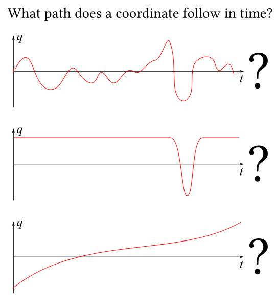
Now, we want to know what the system does as time advances. This amounts to knowing the state of the system for every single point in time.
There are lots of possibilities for what a system might do. The double pendulum might swing up and hold itself horizontal forever, for example, or spin wildly. We call each one a path.
Because the generalised coordinates tell apart all the different states of the system, a path amounts to a value of each generalised coordinate at every point in time.
OK. The point of mechanics is to find out which of the many imaginable paths the system/each coordinate actuallytakes.
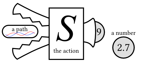
The Action
To achieve this, Lagrangian mechanics says the system has a mathematical object associated with it called the action. It’s almost always written as \(S\).
OK, so here’s what you do with the action: you take one of the paths that the system might take, and feed it in; the action then spits out a number. (It’s an object called a functional, to mathematicans: a function from functions to numbers).
So every path the system takes gets a number associated with it by the action.
The actual numbers associated with each path are not actually that useful. Rather, we want to compare ‘nearby’ paths.
We’re looking for a path with a special property: if you add any tiny little extra wiggle to the path, and feed the new path through the action, you get the same number out. We say that the path with this special property is the one the system actually takes.
This is called the principle of stationary action. (It’s sometimes called the “principle of least action”, but since the path we’re interested in is not necessarily the path for which the action is lowest, you shouldn’t call it that.)
But why does it do that
The answer is sort of, because we pick out an action which produces a stationary path corresponding to our system. Which might sound rather circular and pointless.
If you study quantum field theory, you find out the principle of stationary action falls out rather neatly from a calculation called the Path Integral. So you could say that’s “why”, but then you have the question of “why quantum field theory”.
A clearer question is why is it useful to invent an object called the action that does this thing. A couple of reasons:
the general properties actions frequently make it possible to work out the action of a system just by looking at it, and it’s easier to calculate things this way than the Newtonian way.
the action gives us a mathematical object that can be thought of as a ‘complete description of the behaviour of the system’, and conclusions you draw about this object - to do with things like symmetries and conserved quantities, say - are applicable to the system as well.
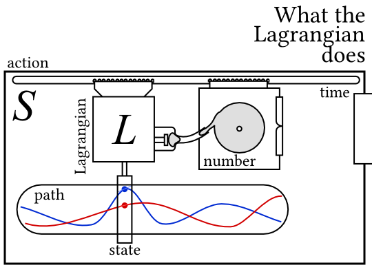
The Lagrangian
So, OK, let’s crack the action open and look at how it’s made up.
So “inside the action” there’s another object called the Lagrangian, usually written \(L\). (As far as I know it got called that by Hamilton, who was a big fan of Lagrange.) The Lagrangian takes a state of the system and a measure of how quickly its changing, and gives you back a number.
The action crawls along the path of the system, applying the Lagrangian at every point in time, and adding up all the numbers.
Mathematically, the action is the integral of the Lagrangian with respect to time. We write that like $$S[q]=\int_{q(t)} L(q,\dot{q},t)\dif t$$
What can you do with a Lagrangian?
Lots and lots of things.
The main thing is that you use the Lagrangian to figure out what the stationary path is.
Using a field of maths called calculus of variations, you can show that the path that stationaryises the action can be found from the Lagrangian by solving a set of differential equations called the Euler-Langrange equations. If you’re curious, they look like $$\frac{\dif}{\dif t}\left(\frac{\partial L}{\partial \dot{q}_i}\right) = \frac{\partial L}{\partial q_i}$$but we won’t go into the details of how they’re derived in this post.
The Euler-Lagrange equations give you the equations of motion of the system. (Newtonian mechanics would also give you the same equations of motion, eventually. From that point on - solving the equations of motion - everything is the same in all your mechanicses).
The Lagrangian has some useful properties. Constraints can be handled easily using the method of Lagrange multipliers, and you can add Lagrangians for components together to get the Lagrangian of a system with multiple parts.
These properties (and probably some others that I’m forgetting) tell us what a Lagrangian made of multiple Newtonian particles looks like, if we know the Lagrangian for a single particle.
Particles and Potentials (the new RPG!)
In the old, Newtonian mechanics, the world is made up of particles, which have a position in space, a number called a mass, and not much else. To determine the particles’ motion, we apply things called forces, which we add up and divide by the mass to give the acceleration of the particle.
Forces have a direction (they’re objects called vectors), and can depend on any number of things, but very commonly they depend on the particle’s position in space. You can have a field which associates a force (number and direction) with every single point in space.
Sometimes, forces have a special property of being conservative. A conservative force has the special property that
depends on where the particle is, but not how fast its going
if you move the particle in a loop, and add up the force times the distance moved at every point around the loop, you get zero
This is great, because now your force can be found from a potential. Instead of associating a vector with every point, the potential is a scalar field which just has a number (no direction) at each point.
This is great for lots of reasons (you can’t get very far in orbital mechanics or electromagnetism without potentials) but for our purposes, it’s handy because we might be able to use it in the Lagrangian.
How Lagrangians are made
So, suppose our particle can travel along a line. The state of the system can be described with only one generalised coordinate - let’s call it \(q(t)\). It’s being acted on by a conservative force, with a potential defined along the line which gives the force on the particle.
With this super simple system, the Lagrangian splits into two parts. One of them is $$T=\frac{1}{2}m\dot{q}^2$$which is a quantity which Newtonian mechanics calls the kinetic energy (but we’ll get to energy in a bit!), and the other is just the potential \(V(q)\). With these, the Lagrangian looks like $$L=T-V$$and the equations of motion you get are $$m\ddot{q}=-\frac{\dif V}{\dif q}$$exactly the same as Newtonian mechanics.
As it turns out, you can use that idea really generally. When things get relativistic (such as in electromagnetism), it gets squirlier, but if you’re just dealing with rigid bodies acting under gravity and similar situations? \(L=T-V\) is all you need.
This is useful because it’s usually a lot easier to work out the kinetic and potential energy of the objects in a situation, then do some differentiation, than to work out the forces on each one. Plus, constraints.
The Canonical Momentum
The canonical momentum in of itself isn’t all that interesting, actually! Though you use it to make Hamiltonian mechanics, and it hints towards Noether’s theorem, so let’s talk about it.
So the Lagrangian depends on the state of the system, and how quickly its changing. To be more specific, for each generalised coordinate \(q_i\), you have a ‘generalised velocity’ \(\dot{q}_i\) measuring how quickly it is changing in time at this instant. So for example at one particular instant in the double pendulum, one of the angles might be 30 degrees, and the corresponding velocity might be 10 radians per second.
Thecanonical momenta \(p_i\) can be thought of as a measure of how responsive the Lagrangian is to changes in the generalised velocity. Mathematically, it’s the partial differential (keeping time and all the other generalised coordinates and momenta stationary): $$p_i=\frac{\partial L}{\partial \dot{q}_i}$$They’re called momenta by analogy with the quantities linear momentumandangular momentum in Newtonian mechanics. For the example of the particle travelling in a conservative force, the canonical momentum is exactly the same as the linear momentum: \(p=m\dot{q}\). And for a rotating body, the canonical momentum is the same as the angular momentum. For a system of particles, the canonical momentum is the sum of the linear momenta.
But be careful! In situations like motion in a magnetic field, the canonical momentum and the linear momentum are different. Which has apparently led to no end of confusion for Actual Physicists with a problem involving a lattice and an electron and somethingorother I can no long remember…
OK a little maths; let’s grab the Euler-Lagrange equations again: $$\frac{\dif}{\dif t} \left(\frac{\partial L}{\partial \dot{q}}\right) = \frac{\partial L}{\partial q_i}$$Hold on. That’s the canonical momentum on the left. So we can write this as $$\frac{\dif p_i}{\dif t} = \frac{\partial L}{\partial q_i}$$Which has an interesting implication: suppose \(L\) does not depend on a coordinate directly, but only its velocity. In that case, the equation becomes $$\frac{\dif p_i}{\dif t}=0$$so the canonical momentum corresponding to this coordinate does not change ever, no matter what.
Which is known in Newtonian mechanics as conservation of momentum. So Lagrangian mechanics shows that momentum being conserved is equivalent to the Lagrangian not depending on the absolute positions of the particles…
That’s a special case of a very very important theorem invented by Emmy Noether.
The canonical momenta (or in general, the canonical coordinates) are central to a closely related form of mechanics called Hamiltonian mechanics. Hamiltonian mechanics is interesting because it treats the ‘position’ coordinates and ‘momentum’ coordinates almost exactly the same, and because it has features like the ‘Poisson bracket’ which work almost exactly like quantum mechanics. But that can wait for another post.
Coming up next: Noether’s theorem
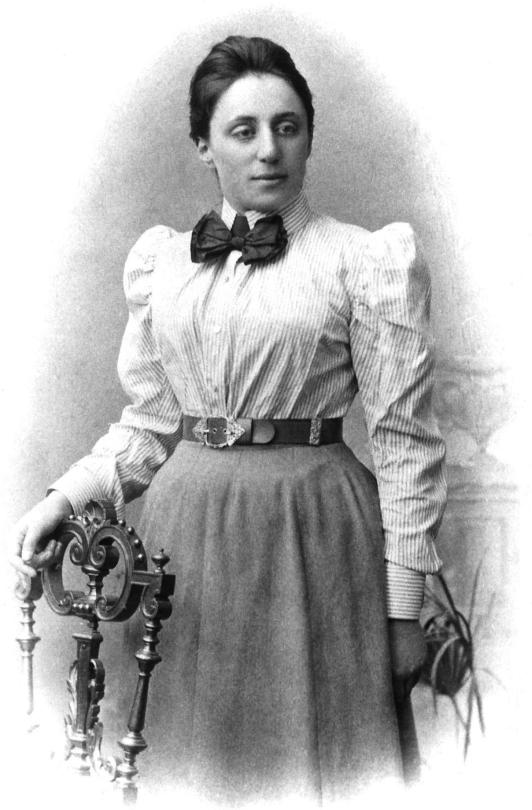
Lagrangian mechanics may be a useful calculation tool, but the reason it’s important is mainly down to something that Emmy Noether figured out in 1915. This is what I’m talking about when I refer to Lagrangian mechanics forming the basis for all the modern theoretical physics.
[OK, I am a total Noether fangirl. I think I have that it common with most vaguely theoretical physicists (the fan part, not the girl one, sadly). To mathematicians, she’s known for her work in abstract algebra on things like “rings”, but to physicists, it’s all about Noether’s Theorem.]
Noether’s theorem shows that there is a very fundamental relationship between conserved quantitiesandsymmetries of a physical system. I’ll explain what that means in lots more detail in the next post I do, but for the time being, you can read this summarybyquasi-normalcy.
Aside from the physics explained, I couldn’t get over the intro
I tried my best to circle what I thought was most, umm, notable
This really is the bestest
I’m really glad people are finding and enjoying this post again!
I’ve copied a lot of my other physics writing to my github site if you’re interested in reading things in a similar vein. Or if you want it on tumblr, try @dldqdot.
I… guess I really shouldn’t be surprised that you’d written a post like this at one point, but (a) it’s neat! and (b) I’ve never actually read your blog on your blog because otherwise I would have known that you have a very neatly organized collection of your major sideblogs.
This is the first of two posts based on a talk given at Dmitriy Bilyk at our probability seminar. I don’t usually go to probability seminar, but have enjoyed Dmitriy’s talks in the past, and I didn’t regret it this time either :)
——
Unsatisfactory Methods
Here is how not to pick a point uniformly on the sphere: don’t pick its polar and azimuthal angles uniformly. This doesn’t work because it will incorrectly bias things toward the poles.
The problem is that this cylindrical trick only works on the 2-sphere. There is no natural notion of “cylindrical coordinates” for higher-dimensional spheres, because how many coordinates do you take linearly and how many do you take as angles?
Bilyk did not say this, but presumably no choice you can make, or at least no consistent choices that you can make for all $n$, such that you get a uniform distribution— otherwise it really would have been a short talk :P
What Bilyk did say is that there are several ways to choose points uniformly from a sphere, but “there are very few deterministic methods”. But before we can tackle these methods, we actually need to answer a more fundamental question: what does it mean to choose deterministically choose points uniformly? Generally “choosing uniformly” means sampling from a constant random variable, but that X is clearly not available to us here.
——
Riesz Energy
One way to go might be to minimize the Riesz energy. Whenever we have a collection of points $Z=\{z_1,\cdots z_N\}$, can write
We see that if the $z_k$ are very close to each other, this energy is going to be large; a set $Z$ that makes the energy small will be one whose points are generally “as far from each other as possible”. Since it’s a sphere, you can’t get too far away, and so there’s an interesting optimization to be done here.
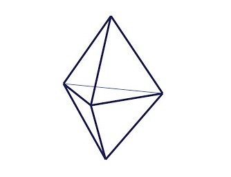
So this seems nice, but there’s a problem. It turns out that minimizing the Riesz energy is just, like, stupendously hard. The best exact result we have was given in 2010, when Schwartz proved that $E_1$ is minimized for $N=5$ (!) by the triangular bipyramid.
To give some indication about why the problem is hard: the triangular bipyramid is not the minimizer for the Riesz energy with $N=5$ for all $s$. It is suspected that it minimizes it for all sufficiently small $s$; but one thing we know for sure that when $s$ gets large enough, the square pyramid is better.
Conjecture. There exists a critical value $s’$ such that for all $1\leq s<s’$, the triangular bipyramid minimizes $E_s$, and for all $s’<s$, the square pyramid minimizes $E_s$.
This conjecture is wide open: we don’t even know that the square pyramid minimizes $E_s$ for any value of $s$!
——
Discrepancy and a Theorem of Beck
Another, rather different way to measure the uniform-ness of a set $Z$ is by computing its discrepancy. The formal definition of discrepancy is really a lot scarier than necessary, so I won’t write it here. The idea is that if you pick any (measurable) set $S$, you can either
calculate the measure of the $S$, or
count how many of the points $z_i$ live inside $S$
Most of the time, these two numbers are going to be different, and the discrepancy $D(Z,S)$ is the difference between the numbers, divided by the number of points in $Z$. But this is not the most useful number because we have this extra data $S$ hanging around; the better idea is to let the discrepancy be the maximum of $D(Z,S)$ over all $S$ (technically the supremum).
Intuitively speaking, that if you were to have a $Z$ for which the discrepancy in the latter sense were small, then $Z$ looks “uniformly distributed”, even if $Z$ is deterministic.
However, measurable sets can look pretty wacky, and so in order to let geometry reign over set theory, it often helps to be a little more refined. Given a collection of sets $\mathcal S$, we say that the discrepancy $D(Z,\mathcal S)$ is the supremum of $D(Z,S)$ over all $S\in\mathcal S$. So it’s basically the same thing as what we did above, except that instead of doing all measurable sets, we only do the ones in the collection.
Figuring out optimal discrepancies is also not very easy, but people have over the years figured out strategies for determining asymptotic bounds. And even that tends to be pretty tough. For instance, if we’re considering things on the sphere, it may seem reasonable to look at $\mathcal S$ the collection of spherical caps:
What is the best available discrepancy in this setting? The answer, morally speaking, is that it’s “close to $1/\sqrt{N}$”, but it has a small dimensional correction:
Theorem (Beck 1984). For any positive integer $N$, there exist positive constants $C_0$ and $C_1$ such that
So you can always find a set $Z$ that does a little better, asymptotically, than $1/\sqrt{N}$; what exactly “a little” means depends on how high-dimensional your sphere is.
——
In the next post, we talk about more recent developments, including a third notion of uniform distribution which will bring us all the way to Bilyk’s work in the present day.
For almost two years, I’ve been skating by, saying “I don’t want to explain homology right now, homology is complicated, ask me later.”.
Later has come, folks. This is the final post of a seven-part sequence dedicated to shining light on this beautiful, mysterious beast. (1234567)
——
The aim of this post is to say some words about cohomology.
It is harder to give an intuitive understanding about cohomology from the cellular perspective. Probably the least algebraic way to introduce cohomology is through de Rham cohomology, but even this relies on an extremely solid grasp of multivariable calculus. It’s unreasonable for me to assume you have such a strong intuition, and frankly mine is not very good either.
However, I can say words to convince you that although we no longer have a geometric intuition, things seem more or less the same:
The two basic notions in cohomology are cocyclesand coboundaries
Coboundaries count for nothing.
Every coboundary is a cocycle, but some cocycles are not coboundaries.
Cocycles and coboundaries are special examples of cochains.
Cocycles which differ by a coboundary are called cohomologous, and are said to be of the same cohomology class.
The collection of cohomology classes is called the cohomology of the space
Breaking the cohomology up by dimension, we obtain the cohomology groups of dimension $\bm{d}$, which we notate $H^d(X)$.
However, this is a bit too brisk to explain why we have a whole separate concept for these two things.
The point of contact between homology and cohomology is at the level of chains: every cochain can be thought of as a chain of the same dimension by a fairly standard operation known as vector space duality. This process is kind of uncomfortable for the (co)chains; there is a meaningful sense in which chains and cochains really “don’t want” to be identified with each other. But we can force it to happen anyway, if we so choose.
However, once you start moving away from chains, the two theories diverge. The most notable difference is that while the boundary of a $d$-dimensional chain is $(d-1)$-dimensional, the coboundary of a $d$-dimensional cochain is $(d+1)$-dimensional! By the time we get to the level of homology groups, it seems like the two theories are hopelessly different.
But then, a miracle occurs: for the most reasonable class of $n$-dimensional spaces, $H_d(X)$ and $H^{n-d}(X)$ are essentially the same— for instance, they contain the same number of (co)homology classes. This miracle was first discovered by Poincaré, and it uses a much more natural method of assigning chains to cochains, thus, today this phenomenon is called Poincaré duality.
[ Now, nothing comes for free in this world, including the “naturality” of Poincaré duality. The cost is that this duality does not take $d$-chains to $d$-cochains, but instead takes $d$-chains to $(n-d)$-cochains. ]
——
Poincaré duality is really cool! But, stealing a line from Ghrist’s Elementary Applied Topology: “The beginner may be deflated at learning that cohomology seems to reveal no new information… Students may wonder why they should bother with this… as it is alike to homology in every respect except intuition.”
Indeed, Poincaré duality is almost too much of a good thing; were it not for a second miracle, cohomology may have been relegated to a footnote in the algebraic topology historybooks. And the second miracle is this: while homology classes naturally “want” to be aggregated by dimension, cohomology classes do not. The collection which I called the “cohomology” in the list above is more commonly known as the cohomology ring.
[ Briefly, this is because cochains are actually functions. Such functions can be multiplied, and this product structure provides the “glue” that binds the (direct sum of the) cohomology groups together as a ring. ]
You may be surprised to see the word “ring” showing up here. In this context it roughly means “number system”: two elements of a ring can be added together or multiplied together. Rings are a central object of study in the field of algebra proper, and so a great deal of general theory can now be imported into this situation, making cohomology a secret trove of structure hidden deep, deep beneath the geometry of the space.
For almost two years, I’ve been skating by, saying “I don’t want to explain homology right now, homology is complicated, ask me later.”.
Later has come, folks. This is the sixth post of a seven-part sequence dedicated to shining light on this beautiful, mysterious beast. (1234567)
This post will be a little bit long, because I didn’t see any point in belaboring this calculation into multiple posts. You won’t need to have seen anything from this calculation to read the final post, so if you get impatient you can feel free to move on.
——
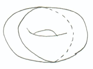
Meet the Torus
We have built so much so far out of one-dimensional examples, that I feel obligated to show you at least one interesting two-dimensional hole. A natural example is provided by the torus, which you can think of as the crust (so: hollow) of a donut:
A few remarks before proceeding:
I will do my best to illustrate what is happening here, but since we are now looking at a curved two-dimensional surface, it becomes harder to see what’s happening in a drawing. It would probably help if you actually got a donut (and if not, at least you now have a donut! Yum!)
I will draw some grid lines on the surface of the donut, and I will try to draw them lightly so we do not mistake them for one-dimensional chains.
Finally, it is common parlance in mathematics to remove the word “dimension” whenever possible. For instance, $1$-dimensional chains are called $1$-chains, $2$-dimensional cycles are called $2$-cycles, and so on. \item One that is a bit confusing: a $2$-boundary, for instance, is a $2$-chain, and also the boundary \emph{of} a $3$-chain. So the dimension refers to the dimension of the shape itself, not the dimension of the thing which the shape is the boundary of.
Let’s begin by looking at $2$-cycles. This is not something we had ever considered before, but we will do so now. Actually, there are not many options available to us. One $2$-cycle is the entire surface itself. This has the right dimension and it is a cycle (make sure to convince yourself that it is, indeed, boundaryless). It is, in fact, the only one!
Here is an argument to see why: suppose we wanted to make a $2$-cycle. It would need to contain at least one point, and so in order to have the right dimension, we would need to have some small disk.
However, this disk has a boundary. If we make the disk smaller, we’ll never totally get rid of the boundary, so let’s try to make it larger instead. In order to remove the “upper part” of the boundary, we have to wrap around the torus one way…
… and then to get rid of the rest of it, we have to wrap around the other way:
(Note: this picture obviously still has a boundary; in order to make it disappear we have to keep wrapping the chain around the torus. In the end, the two boundaries will meet up, at which point they cease to be boundaries at all, and the chain is the entire torus, which is what we were expecting.)
Now, is this $2$-cycle a boundary? Remember that this means it would be a $2$-boundary, or in other words the boundary of a $3$-chain. But a moment’s consideration makes us realize that it could not possibly be the boundary of a $3$-chain: the space is itself only two-dimensional! There’s not enough room to fit a $3$-dimensional shape into it.
——
Dimensional Downstep
Having handled the $2$-dimensional case, we now move to the harder task of classifying $1$-cycles. We will not be so lucky to just be able to count cycles this time: there is lots of room for us to put loops into the space.
It’s hard to explain, but hard to unsee, that a $1$-cycle is going to be a $1$-boundary unless it “wraps around” the torus somehow: this makes sense with our intuitive definition because it seems like there is a hole in the center:
(In this drawing it kind of looks like you could find a $2$-chain that $\alpha$ is the boundary of. But the dashed part of $\alpha$ is on the back of the torus: if you try to “fill in” the shape you end up on the wrong side of the space.)
In that diagram, you can actually already see another $1$-cycle: all of the grid-lines are 1-cycles! It’s easy to see that the parallel ones are all homologous to each other (take the “rectangle” in between them). It’s less obvious is that none of the “long” ones are homologous to the thickly-drawn $1$-cycle, but this is also true.
We can also see this geometrically, although it is even trickier: notice that $\alpha$ has only one point of intersection with any grid line $\beta$. This poses a problem if we try to find a $2$-chain with boundary $\alpha-\beta$ (which, remember, is also $\alpha+\beta$), because it ends up needing to fill the whole torus:
But we already know that the torus is a $2$-cycle, hence boundaryless, so it couldn’t possibly be that the boundary is $\alpha+\beta$. Therefore, $\alpha$ and $\beta$ cannot be homologous cycles.
——
The One that Got Away
It is natural, at this point, to believe we are done (except that we haven’t mentioned the cycles which are boundaries— now we have). But if we do the calculation for the number of holes, we find that there is an issue. We have $\alpha$ is in a different homology class from $\beta$, and so we’ve found that there are $3$ homology classes (including the class of boundaries). This is a big problem, because $3$ is NOT a power of $2$: It isn’t $2$, and it isn’t $4$ either! We must have missed a cycle.
Indeed we have: I will spare you the trouble of finding it yourself.
But this “missing cycle” raises a more serious concern. How do we know we didn’t miss anything else? Are we absolutely sure there aren’t secretly some more classes hiding around somewhere?
It would surely be impossible to go around checking every single loop: What if you wrap around the center hole four times and then cross the gridline? What if you do the third cycle, but don’t quite close, and then wrap around the center hole and then do the third loop again and then…?
I’m sure that it would be possible to come up with a visual argument like the one I gave above, but you would have to be extremely clever to find it (I do not know one, myself). The point is that when we look at any space that’s even a little bit complicated, it’s not so easy to know when you’re done.
It turns out that there is a method for knowing when to stop counting as well. Unfortunately, that method is quite technical, and this technicality seems to be unavoidable. Actually, the main reason that I delayed writing this sequence so long is because I was trying to find an intuitive way to describe this method; I have not been able to do so. Taking the time right now to build up the required machinery would more than double the length of this sequence, so I am not going to do that. (I am strongly considering writing another sequence, although there is not too much time left >.<)
The final post is a more of an epilogue, which will talk about the highlights from the story of homology’s hotshot cousin: cohomology.
This post represents the second half of a talk given by Emine Yildirim at our combinatorics seminar.
If you’ve not already read the first one, you don’t technically have to, as long as you’re happy assuming that there are special posets associated to each Coxeter group called “cominiscule”. But it will probably be more rewarding if you read the posts in order.
In any case, this post will make really no attempt at all to be elementary.
——
Excuse Me, Which Algebra?
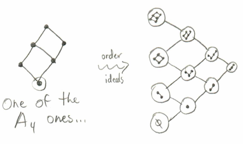
We wish to consider a path algebra, and so we need to have a directed graph. You might imagine that we would just use the Hasse diagrams of the posets which we just drew, with some orientation thrown on. That’s a very reasonable guess; it just happens to not be what Yildirim did.
Instead she first considers the set of order ideals (which are all subsets of poset elements which are “downward closed”: if $x$ is in the subset then every $a\leq x$ must also be in the subset) of a cominiscule poset. Since order ideals are, in particular, subsets of the same set, the collection of all order ideals come with their own natural order structure— namely, inclusion of sets.
[ Eagle-eyed viewers may notice what one of the members of the audience pointed out: this poset structure is actually a cominiscule poset itself (for type C). After some consideration, we decided that this is probably a coincidence; the order ideal poset of cominiscule posets will not in general be cominiscule. ]
We take the Hasse diagram of that poset (e.g. as drawn above), interpret it as a graph with the edges as directed downward, and finally take the path algebra of that(whew!). We will call such an algebra $\mathcal A$, suppressing the dependence on the cominiscule root. Note that this directed graph is acyclic, and so $\mathcal A$ is finite-dimensional.
In any case, the goal is to prove the following:
Conjecture. The Auslander-Reiten translation $\tau$ has finite order $2(h+1)$ on the Grothendeick group of the bounded derived category of $\textbf{Mod}(\mathcal A)$.
So there’s lots of words here but the point is that that Yildirim was able to prove this conjecture for all the cominiscule posets… except the triangular poset that comes from types C and D. So it’s technically still a conjecture, but she solved a substantial portion of it, and so I will still refer to “Yildirim’s proof.”
In the remainder of the post, we make an attempt to explain why this might be true, and why the Coxeter transformation has anything to do with anything.
——
“Bounded Derived Category”?
I will not attempt to define the bounded derived category construction, but I will tell you an important fact abut it: it is “derived” in the sense that its objects are chain complexes $\to A \to B\to C\to$, but all of the quasi-isomorphisms are invertible.
This bit of abstract nonsense means that we can replace any $\mathcal A$-module $M$ by its minimal projective resolution:
[ Here we are using the “homological” definition of a projective resolution, where $M$ does not show up in the sequence itself but rather is isomorphic to the kernel of the last map. It’s not super important. ]
In the post based on Yildirim’s pre-talk, we pointed out that the defining characteristic of the Coxeter transformation is that it “turns projectives into injectives”. One can define the Coxeter transformation so that it does this functorially, i.e. in such a way that we get a sequence
This turns out to be an injective coresolution of any module $N$ (“co” meaning that $N$ is the of the kernel of the second map), and we say that the Coxeter transformation turns $M$ into $N$.
Update: actually things are even worse than I thought: in general this does not even have to be an injective resolution! (Thanks @yildirimemine (!!) for the correction.)
——
The Key Lemma
The Coxeter transformation is a useful tool for understanding the Auslander-Reiten translation $\tau$, but there is a major hurdle to making it any more useful than just using $\tau$ itself.
A module $M$ of a path algebra coming from a Hasse diagram is called an interval if it arises as a quiver representation in the following way:
choose an “upper” vertex $\beta$ and a “lower” vertex $\alpha\leq\beta$,
for each vertex $v$ between these two, i.e. satisfying $\alpha\leq v\leq\beta$, place a copy of the field $k$ at $v$, and
place the zero map at every edge between any two vertices.
Then the Coxeter transformation need not take intervals to intervals.
However, Yildirim’s proof of the conjecture relies on the following discovery.
Lemma. For all $\mathcal A$ except the one arising from the triangular poset, there exists a collection of intervals which are taken to intervals. Moreover, these form a basis for the (relevant) Grothendieck group.
Again these are words, but they have a practical effect. Namely, any module $M$ can be broken down into pieces, each of which is an interval that is taken to an interval. So, roughly speaking, as long as we understand the Coxeter transformation on such modules, we understand the Coxeter relation in general.
[ In light of the Update, this becomes even more remarkable: some intervals are not even taken to resolutions! And yet somehow there is this nice collection we can carve out that not only is taken to resolutions, but even resolutions of intervals…]
Because of this, and because of the Coxeter transformation’s close connection to the Auslander-Reiten translation, she is able to understand the latter in a more stripped-down form, without its full algebraic trappings. This, finally, she uses to prove the conjecture. The difficulty with the single remaining family of posets is that we do not (yet?) have such a basis.
We had an interesting discussion in our algebra department yesterday, about this innocuous-looking equation. I suggest you don’t try it, unless you’re equally happy with negative integer solutions or know something about elliptic curves!
As it turns out, the smallest positive integer solution has 80-digit numbers! Hence you won’t find these using brute-force computer searches without some insight on elliptic curves. If you want to read more about the mathematics behind this equation, read this delightful post on Quora by Alon Amit.
“You may have seen such meme images before. They are always pure click-bait garbage: “95% of MIT graduates couldn’t solve this!”, where “this” is some inane, or ill-defined, or trivial brain teaser.
This one is not. The meme is a clever, or wicked, joke. Roughly 99.999995% of the people don’t stand a chance at solving it, and that includes a good number of mathematicians at leading universities who just don’t happen to be number theorists. It is solvable, yes, but it’s really, genuinely hard.”
#the quora post is excellent
SECONDED
(In addition to providing a solution whose only incompleteness is that it omits most of headache-inducing transformation formulae, it also includes a rather extensive history of the problem… which confirms that it is indeed a wicked joke.)
So, for reasons [explained below the break*], it occurred to me that the deadline for submitting abstracts to the Joint Meetings is probably pretty soon (it is— September 26— so if you’re planning to submit, better get your ass in gear!). And while I was looking through the sessions, I was once again reminded why I flinging love the Joint Meetings.
Here are some actual titles of sessions— sessions!There will be multiple talks on these things!
AMS Special Session on Set-theoretic Topology (Dedicated to Jack Porter in Honor of 50 Years of Dedicated Research)
MAA Session on Philosophy of Mathematics as Actually Practiced
Short version for the unaware: there has recently been a growing trend in philosophy of mathematics to shift the discipline closer to studying the practices of professional mathematicians.
This is basically everything I like about philosophy plus everything I like about anthropology/sociology (I’m really bad at distinguishing the two) thrown together into a big pot and seasoned liberally with modern math; delicious!
AMS Special Session on Alternative Proofs in Mathematical Practice
Besides just being generically interesting, the title of this session is based on the title of a book that came out recently (which is really darn expensive, sorry). So I’m interested to see how the session interacts with that.
MAA Session on Good Math from Bad: Crackpots, Cranks, and Progress
AMS Special Session on A Showcase of Number Theory at Liberal Arts Colleges
This one’s a little subtle. If this were by the MAA, this would be whatever. But it’s not: it’s by the AMS. This is very outside the usual AMS fare and I’m hoping that it succeeds because that would indicate that at least one of teaching, undergrad research, and non-R1 research are being actively supported by both major American mathematical communities, which… fucking finally.
And then there are all the the sessions I’m excited about because people! Math friends!
AMS Special Session on Research from the Rocky Mountain-Great Plains Graduate Research Workshop in Combinatorics
:Ditme! (we already presented our stuff at last year’s JMM, so it won’t actually be me. but still)
AMS Special Session on Research in Mathematics by Early Career Graduate Students
People like me except marginally better at not procrastinating? yes please?
(Also it’s an AMS Special Session so there’s definitely some expectation of quality there… at least with the work. With the presentation style… we’ll see.)
AMS Special Session on Special Functions and Combinatorics (in honor of Dennis Stanton’s 65th birthday)
MAA Project NExT Lecture on Teaching and Learning — Changing Mathematical Relationships and Mindsets: How All Students Can Succeed in Mathematics Learning by Jo Boaler
NO FUCKING WAY
Jo Boaler is a relentless advocate of IBL techniques in the K12 setting
And in particular wrote What’s Math Got To Do With It? that book was my bible on math ed for a good three years, dam.
AMS Invited Address — Algebraic Structures on Polytopes by Federico Ardilla
* So an idea I’ve had kicking around for a little while is that maybe I could try to take some of the lessons that I’ve learned from writing this blog and give a little contributed talk at the Joint Meetings this year. I’ve never really thought to do this earlier because it just doesn’t feel right to eat up a spot just to do some cheap advertisement. But I think I’m more comfortable with the idea now, since I’ll be several months out from writing the blog by then, and I don’t have a follow-up project planned. I mean, I do, it’s called “writing my damn thesis already”, but I haven’t figured out how to publicize that yet* :P
Part of the reason I want to do this is definitely because I’d love the blog to “count” for something CV-wise, and a contributed presentation at a conference isn’t much but it isn’t nothing.
But another reason is that over the course of my writing OTAM is that I’ve talked with a lot of people in real life who speak longingly about blogging. It’s something they’ve wanted to do for a while— maybe they even did do it for a month or two— but have never really found the time/drive/whatever. And I’ve never really had anything useful to say to comments like this. I think that the effort of preparing a conference talk might force me to straighten out my perspective on the value of this whole enterprise, which I think would allow me to have more meaningful conversations.
(This sounds rather falsely noble, but it’s also a bit self-serving: I suspect that I’ll find myself being one those people ten years from now, if not for blogging then for something else. It would be nice to have something of value to say to future-me, too.
[ * I thought pretty seriously about streaming thesis work. But in the end I came to the conclusion that I would need a much more flexible camera setup so that I could film my paper, or alternatively to get some kind of comfortable whiteboard setup in my room. The issue is that it’s easy to stream TeX, but I can’t do all my actual work in TeX; I need some flexibility to draw faster than I can TikZ. So I got myself a cheap tablet (and wow, that’s a story: ask me about it IRL sometime) thinking that I could get used to drawing on that. But in the end I really just couldn’t; I haven’t figured out how to think on the tablet the way I can think on paper or whiteboards**. I have no doubt that I could learn to do it, but I also have no particular interest in learning right now. ]
[ ** Unpopular opinion: chalkboards are great for teaching and giving talks, but when I do math that I have to actually think about, whiteboard every time. ]
For almost two years, I’ve been skating by, saying “I don’t want to explain homology right now, homology is complicated, ask me later.”.
Later has come, folks. This is the fifth post of a seven-part sequence dedicated to shining light on this beautiful, mysterious beast. (1234567). This is a very important post for us, since we have built up all the background and we will finally see how to use homology to determine the number of holes in a space!
——
Recall that in the last post we gave an algebro-geometric justification which permitted us to understand these two cycles as “essentially the same”:
We thought this was a good thing because both $A$ and $B$ “surround the same hole”, and we only want to count each hole once.
Motivated by this argument, we make the following definitions. If the difference* $A-B$, between two cycles $A$ and $B$, is a boundary, we say that the cycles are homologous, or in other words that they are of the same homology class. This allows us to define the homology of a space as the collection of all homology classes.
Since cycles of different dimensions look qualitatively different, and so they probably surround different-looking holes, it’s natural to want to split up the homology by dimension. We say that the collection of homology classes having dimension $d$ is the $\mathbf{d}^\textbf{th}$ homology group, and is usually written $H_d(X)$, where $X$ is the space in which the chains live.
[ There’s a technicality here: how do we define the dimension of a homology class? After all, homology classes aren’t curves or surfaces or anything; they’re these giant unwieldy collections of many, many chains. However, this “issue” turns out not to be, because any two homologous chains have the same dimension. (This is not totally obvious; it’s worth the effort to draw a picture or two to convince yourself.) Because of this, we can define the dimension of a homology class by determining the dimension of a cycle of that class: any choice will give the same number. ]
[ * You may wonder why I said “difference” instead of “combination”, since $A+B$ and $A-B$ are the same thing, after all, and the former is more geometrically intuitive. The answer is that the subtraction definition works even outside of characteristic $2$; the addition definition does not. ]
——
However, even restricting our attention to a single homology group, we’re still not counting holes quite yet! The number of $d$-dimensional holes in the space is actually not the number of $d$-dimensional homology classes. For instance, when $d=1$, we can use a slight variant on our example space: instead of a disk with one hole, take a disk with two holes. See if you can convince yourself that no two of these four loops are homologous.
[ You may be concerned with the innermost square loop: this is the class containing the boundaries. We include it for the same reason we include zero as a number: it’s true that boundaries count for nothing, but nothingness, itself, counts for something. We make this convention for convenience, because it makes the theory nicer (like, way nicer, you’d actually be amazed); this is exactly the same reason that we consider zero to be a number. ]
You can keep playing this game: if there are three holes, the picture looks like the one below. (Despite my best efforts, this picture kept turning out a mess; this one I think is at least somewhat legible):
So it turns out that, if you include the class containing all boundaries, the number of classes in a homology group is always a power of $2$; if that number is $2^h$, then we might say that the space has $h$ holes of the corresponding dimension.
By the way: If you think the $2$ in $2^h$ has something to do with being in characteristic $2$, you’re right! But there is also another way to explain it, which perhaps lines up more reasonably with the picture.
People with more advanced mathematics backgrounds may know that $2^h$ is the number of elements in the power set of a set of size $h$, or in other words, is the number of subsets. Applying this knowledge to the situation at hand, it stands to reason that a homology class consists of loops which surround a particular collection of holes. If you believe that the chains I’ve chosen for the pictures above represent “typical” members of their homology classes, then this probably makes sense :) For instance, the fourth cycle in the two-holed space represents the collection “both holes”, and the little squares in both spaces represent the “empty collection” of holes.
——
We’ve made it!
We have described holes, things which “aren’t there”, with genuinely intrinsic features of the space. This was no small feat, and it is worth celebrating.
If this is all you know about homology, you’re in a pretty good place (at least as far as not-being-freaked-out-when-it-gets-mentioned goes). However, we may wish to see some more interesting examples. In the next post, we will grant that wish by peering into some higher-dimensional holes.