#engineering


I 3D printed this elephant to hold my glasses when I put them down, hebis pretty good at it.
How cool: An eight year-old came home from a science class she was taking and felt so empowered by all the experiments she got to conduct that she wrote a song about it.
Sit back, relax, and enjoy!
Let’s look in detail at the process of boiling a pure substance.
We’ll start out with a compressed liquid. We’ll say it’s water at 25 deg C. Moreover, let’s say it’s contained in a cylinder with a piston so that the pressure inside the cylinder is always at atmospheric pressure.
If we start heating up the cylinder, the water inside will expand slightly. The pressure will remain constant as the piston moves with the water’s expansion. Once we get to 100 deg C, the water exists as a saturated liquid - any additional heat will cause it to vaporize.
If we keep adding heat to it, things get interesting. The water will start to boil. It’s volume will increase drastically, but its temperature will remain the same. All the energy you’re putting into it is going into the phase change. The amount of energy it takes to go from a liquid to a vapor is called the latent heat of vaporization. (Similarly, the amount of heat it takes for a solid to melt into a liquid is the latent heat of fusion.) So while the water in your cylinder is in the process of boiling, it exists as a mixture of saturated liquid and saturated vapor. Its temperature will remain at a constant 100 deg C throughout the process. Although its apparent volume will increase, its specific volume - the volume per unit mass - will also remain constant.
Once all the water has been vaporized, if you continue adding heat to the cylinder, the water will start to rise in temperature again and its specific volume will start to increase. In this state, it exists as a superheated vapor.
The entire process we just described looks like this.
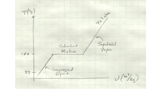
Note that this show temperature vs. specific volume for only one pressure - if we varied the pressure as well, things would look quite different. The interdependence of temperature, volume, and pressure will be important in our analysis of thermodynamic processes.
We’ve spent some time going over the basics of heat enginesandrefrigerators. These are machines which manipulate a working fluid through some sort of cycle in order to move heat from one location to another. We have some idea of the overall way they work, but to really understand the details of what’s going on, we’re going to have to know a little more about how this working fluid behaves.
For right now, we’ll restrict our discussion to materials which qualify as pure substances. A pure substance has the same chemical composition throughout - all its molecules are the same. We’re all familiar with phases of matter - solid, liquid, and gas are the ones we see on a daily basis. Matter in solid form has its molecules arranged in a regularly structured lattice. In a liquid, molecules have about the same distance from each other as they do in a solid, but they’re not held in a structure and can move around each other freely, although their close spacing means that intermolecular forces play a large part in their motion. In a gas, molecules are widely spaced and careen about as they please, interacting with each other only through collisions.
For thermodynamics-related purposes, we’re really interested most in liquids and gases. Controlling the transition between these two states is the key to moving a lot of energy around. So let’s define some terms.
Acompressed liquidorsubcooled liquid is one that is in no danger of vaporizing.
Asaturated liquid is one that is about to vaporize.
Asaturated vapor is one that is about to condense.
Asuperheated vapor is one that is not in any danger of condensing.
Distinguishing between these is important from a thermodynamics because a fluid will have different properties related to its ability to absorb and release energy in each state. In coming articles, we’ll look a little more closely at the exact process of transition between phases.
We’re going to be looking more closely at amplifiers in the coming weeks. The specifics of how an amplifier is built can get pretty complex, so we’re going to want some kind of model that approximates the overall behavior of an amplifier and is simple enough for us to analyze relatively easily. Here’s a general one we can use:

This looks like a mess at first, but when you break it down, it’s not so bad. The left side is the input to the amplifier. v_s is the signal coming in. C_in and R_in represent the input impedance to the amp - that is, the impedance the signal sees on its way in. v_in is the signal the interior workings of the amp actually sees.

The right side is the stuff coming out of the amp. The triangle on the left is an imaginary voltage source that stands in for a lot of complicated amplifier stuff for us. All it does is produce a voltage equivalent to v_in multiplied by some internal gain, g. C_o and R_o here represent the output impedance of the amplifier.

We’ll be doing a lot more with this model and others like it.
We’ve met amplifiers before in the form of op-amps. We’re going to see a lot more of them. In general terms, an amplifier makes a small signal bigger. But there’s some subtlety to this: not all signals are created equal. We’ve been looking at the effects of frequency on impedance, so we know that a signal of the same frequency will behave differently going through a capacitor than it will going through an inductor or a resistor. With what we know now, we have the power to create amplifiers that selectively boost some frequencies and attenuate others.
Let’s think a little bit about what this kind of amplification looks like. The kind of amp we’re all familiar with is an audio amp. If you’re amplifying an audio signal, you want all the stuff within human audible range (about 50 Hz - 15000 Hz) to be amplified equally. So the frequency response for your amplifier might look something like this:

A couple of things to notice about this graph. Gain is a unitless number describing the ratio of the output to the input. So a gain of 100 means the strength of the output is 100 times the strength of the input. The equation below shows a voltage gain, but you can also talk about other kinds of gain.

Note also that the frequency axis on the graph above is one a log scale. At the range of frequencies we’ll commonly be dealing with, this is a necessity just due to space constraints, but we’ll see later on that logarithmic graphs can give us some interesting insight into amplifier behavior.
So the amplifier in the graph above boosts signals within a range of about 50 Hz to 15 kHz more or less equally. It’s not perfect - you lose a little at the extreme high and low ranges, but there’s a solid midband letting most of the frequencies of interest come through. Suppose you wanted to boost the bass of your audio. Bass frequencies run about 40 Hz - 400 Hz. Your amplifier frequency response in this case might look like this:

You might do this by chaining two amplifiers one after the other - one for the bass, one for the rest of the signal range. We’ll look more closely at the specifics of how to make and analyze these in the coming weeks.
Perpetual motion machines are a perennial staple of fringe science. Many of them are very clever and seem, at first glance, as if they should work. If they did work, they would violate the laws of thermodynamics - you’d be getting energy for free. This video walks through a few simple ones and shows how they work. (Or don’t work.)

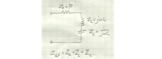
So let’s take a quick look at how varying frequency changes the performance of a circuit. The circuit above has a capacitor, inductor, and resistor in series. We’d like to know what the output, Vout, is as a function of frequency.
We can get Vout just as we’d normally do with a voltage divider. Since we’re dealing with inductors and capacitors, frequency will show up here.

We can manipulate this a little to get it into the standardized form we looked at earlier and make the substitution of s for jω. We’re left with an equation that describes the behavior of Vout with regard to frequency.

Post link
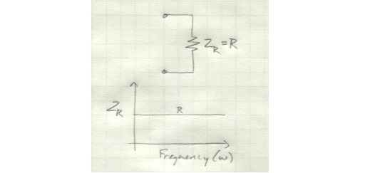
We’ve spent a lot of time talking about the impedance of resistors, capacitors, and inductors. We know that the impedance of inductors and capacitors is dependent on frequency, but we haven’t really explored what that means.
A resistor presents the same amount of resistance regardless of frequency.
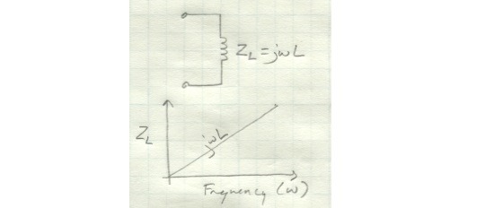
For an inductor, the impedance increases linearly as frequency increases.
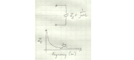
For a capacitor, the impedance decreases rapidly as frequency increases.
So what about a circuit which includes all three elements? Its combined impedance will be the sum of the individual impedances. You’ll get an overall impedance that is high at very low frequencies, becomes low at a slightly higher frequency, and then gradually increases again.
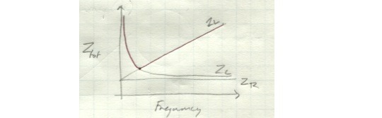
In other words, this thing is basically a filter that blocks very high and low frequencies and lets signals of lower-midrange frequencies through with relatively little difficulty.
If we rearrange equation a little, we get something that’s kind of ugly, but fairly compact. We’ll substitute s for jω - we’ll talk about why later on, but for now, just know that s=jω. We’ll be seeing a lot more of this equation in future articles.

We’ve talked about the second law of thermodynamics as the idea that energy naturally flows from a point of high potential to low potential. There are a couple of other ways you can think about this.
One is called the Kelvin-Planck statement of the second law:
A device which operates on a cycle cannot exchange heat with a single heat reservoir and produce a net amount of work.
Compare this to the heat engine we looked at earlier. A heat engine schematically looks like this:
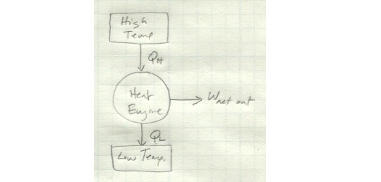
It exchanges heat with both a high- and low-temperature reservoir and produces a net amount of work. If instead it only exchanges heat with a single reservoir, it looks like this:
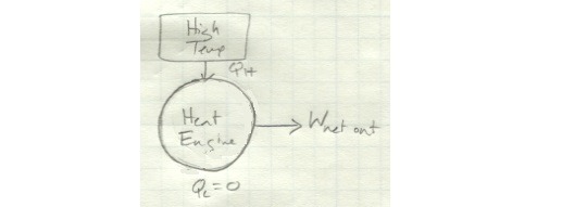
Looking at it like this, you see clearly why this is impossible: in this schematic, there is no Q_L - all of the heat coming in is converted to work. In other words, this device has 100 percent efficiency - something we know can’t happen.
Another formulation of the second law is the Clausius statement of the second law:
A device which operates on a cycle cannot move heat from a lower temperature reservoir to a higher temperature reservoir as its only effect.
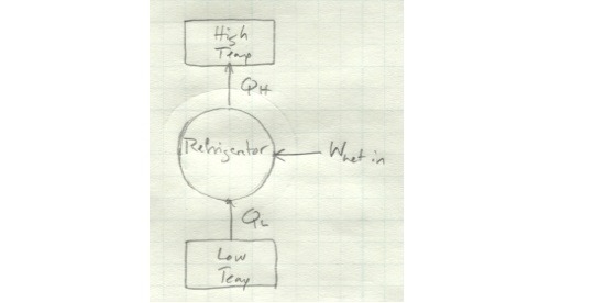
This one also becomes clear if we look at it schematically. Here’s a regular refrigerator schematic:
And here’s a refrigerator which violates the Clausius statement:
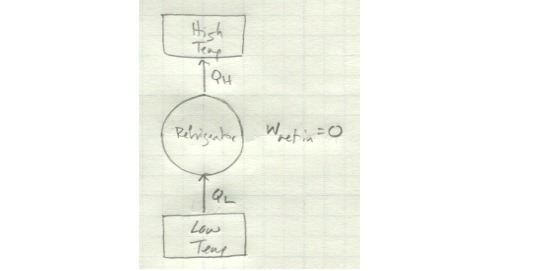
There’s no net work input here, so the energy taken in as Q_L magically increases in quality to be output as Q_H without any other energy input.
Note that all of these formulations of the second law can be expressed mathematically in the same way: Q_H is equal to the sum of Q_L and W_net.

If you have a device in which any of these terms are zero, something is wrong.
We’ve spent some time on the second law of thermodynamics - energy flows naturally from high potential to low, from hot to cold. Most of us have refrigerators or air conditioners in our dwellings - devices which seem to violate this law. They somehow move heat out of a colder space and into a hotter space. So what is going on here?
The short answer is that the refrigerant in these devices acts as a temporary energy storage medium - by some clever manipulation, we can move the refrigerant through a cycle such that at the point it travels through the space we want to cool it absorbs energy, which it needs to dump when it gets to the warmer exhaust space.
Here’s a typical refrigerator schematic.

Refrigerant enters the compressor as vapor. The compressor does work to increase its pressure. Increasing its pressure also increases its temperature, so by the time it hits the condenser it’s relatively hot. In fact, it’s hot enough relative to the surrounding environment that it sheds heat as it flows through the condenser. By the time it leaves, it’s condensed and much cooler, although it’s still at a very high pressure. It goes through an expansion valve from here, which drastically drops both its temperature and pressure. So it enters the evaporator as a low temperature, low pressure liquid. In this state, it is low enough energy that it absorbs energy from the surrounding environment going through the evaporator. When it leaves, it’s a vapor again, ready reenter the compressor and start another cycle.
This works because we are injecting energy into the cycle in the form of work done by the compressor in order to get the refrigerant to a state where the heat it absorbed from the refrigerated space can be dumped to the outside environment.
We’ve been talking about step-down transformers that can convert between a high line voltage and more moderate local voltages. You might be asking yourself why we need to do such a thing in the first place. Why can’t we just transmit utility power at 120 V or 240 V?
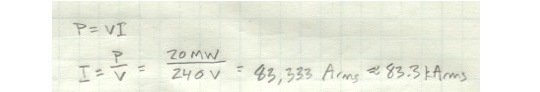
All right, let’s try it. Say we need to transmit 20 MW of power over a 100 km. If we do it at 240 Vrms, we’ll have a current of 83.3 kArms flowing through the conductor.
Some of the 20 MW we’re transmitting is going to be lost - that is, dissipated as heat. We’d like to minimize losses, so let’s say we’re aiming for 97% efficiency - no more than 3% of that 20 MW lost. Since power dissipated is a function of current and resistance, we know we’ll need a conductor with an overall resistance of 8.64 x 10^-5 Ohms over a distance of 100 km.

The resistance of a conductor is a function of its length, l, its cross-sectional area, A, and the conductor’s resistivity, ρ, which is a property of the material it’s made of. We’ll assume a resistivity here of 8 x 10^-8 Ohm-meters. From here, we can figure out what kind of cross-sectional area our conductor needs - in other words, how large the cable’s diameter has to be.
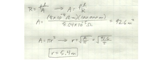
To make this work, you’d need a conductor with a radius of 5.4 m. Clearly, this isn’t going to happen.
If you want a conductor that’s actually practical, that means you need to transmit power at high voltage - since a higher voltage at the same power will result in a lower current, this means your losses will be lower, allowing you to use a much smaller conductor. Here are the same calculations done with a transmission voltage of 240 kVrms instead of 240 Vrms.

In this case, you need a conductor with a radius of about 0.5 cm, which is much more reasonable.

So we’re talking talking about transformers, which are commonly used to step down from the very high voltages present on utility lines to the lower voltages available in a commercial or residential setting. In this scenario, we’re going from a 20 kV line voltage to a 240 V local voltage. We’ll assume that the 240 V off that transformer is supplying 15 buildings with a supply of 150 A each. What kind of turns ratio is needed for this transformer, and how much power does it need to be rated for?
The turns ratio will be the same as the ratio of the voltages between the primary and secondary coils. In this case, it works out to 0.012.

To figure out the power rating, we need to know current and voltage. We know what that is on the secondary side, but the primary side is where it’s really going to be a problem. We know there’s 20 kV on that side, but we don’t know the current. Fortunately, we can figure it out knowing the current on the secondary side and the turns ratio.

We now have the current and voltage present on the primary side. From here, we can get the power by multiplying them together.

Here, the transformer needs to be rated for at least 540 kVA.
Post link
Some of the nuts and bolts behind the navigation of the Apollo spacecraft.

We have a heat engine taking in heat at a rate of 100 MW from a high temperature reservoir. 75 MW of this energy is rejected to a low temperature reservoir. The rest is converted to useful work. How much net work output does this heat engine produce and how efficient is it?
The only source of energy in the system is Q_H, so we know that the energy leaving in the form of W_net out and Q_L must be equal to the energy input, Q_H. Or, put another way, W_net out must be equal to the difference between Q_H and Q_L.
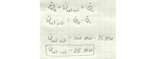
In this case, we get a net work output of 25 MW from this engine.
Efficiency is the ratio of your desired output to your input. In this case, the output we care about is useful work, and the input to the system is Q_H. So we get a thermal efficiency for the engine of 25%.

Post link
Video clearly explaining the second law of thermodynamics and its implications for efficiency.
So a transformer is a device that consists of two magnetically coupled coils. It can be used to step a voltage up or down to whatever level you desire based on the ratio of turns of the coils. For an ideal transformer, this process is lossless - no power is consumed doing this operation. (Real transformers are not so lucky.)
Let’s take a look at a generalized ideal transformer. There’s a primary side, which has some kind of source driving it, and a secondary side, which has no source and is driven entirely by its magnetic coupling with the primary side.

We know that the voltages and currents are related by the turns ratio of the coils.

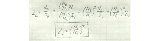
Since we know what the current and voltage are on the secondary side, we can figure out what the load impedance is.

Even though the load impedance is physically disconnected from the primary side, it will still present some impedance to the primary side, since ultimately this is what’s driving it. Like the voltage and current, the actual input impedance the primary side sees, Z_1, will be determined by the turns ratio.
We’ve been talking about mutual inductance and magnetically coupled circuits. If you have a couple of coils of wire adjacent to each other such that they can get caught up in each other’s magnetic fields when a current is run through one or both of them, one coil can induce a voltage in the other, even though the circuits are not physically connected.
This setup is the basic construction for a transformer, one of the most ubiquitous pieces of equipment in power transmission. Just as in the examples we’ve been looking at, a transformer consists of two coils of wire next to each other. In a transformer, they’re both usually wrapped around a magnetic core of some kind. The purpose of this is to channel the magnetic flux so that more of it is caught by the coils and increase the strength of the magnetic coupling between them.

Let’s assume for the moment that this core is perfectly ideal - that it channels ALL the magnetic flux perfectly efficiently, such that the same magnetic flux is experienced by both coils.

If this is the case, then the ratio of the coil voltages is equal to the ratio of coil turns. In other words, you can convert from one voltage to another by adjusting the number of coils in the transformer.

There’s a similar relationship going on with the currents.

If we manipulate these equations a little, we find that the total power of the transformer is zero. (For an ideal transformer, at least.)


GUESS WHO HANDED IN HER DISSERTATION TODAY??? It’s meeeee!!!!


Long study day as I approach the end of my dissertation- so close to the end!