“When you think about government surveillance in the United States, you likely think of the National Security Agency or the FBI. You might even think of a powerful police agency, such as the New York Police Department. But unless you or someone you love has been targeted for deportation, you probably don’t immediately think of Immigration and Customs Enforcement (ICE).
This report argues that you should. Our two-year investigation, including hundreds of Freedom of Information Act requests and a comprehensive review of ICE’s contracting and procurement records, reveals that ICE now operates as a domestic surveillance agency. Since its founding in 2003, ICE has not only been building its own capacity to use surveillance to carry out deportations but has also played a key role in the federal government’s larger push to amass as much information as possible about all of our lives. By reaching into the digital records of state and local governments and buying databases with billions of data points from private companies, ICE has created a surveillance infrastructure that enables it to pull detailed dossiers on nearly anyone, seemingly at any time. ”
“Most Americans probably do not imagine that their information is captured by ICE’s surveillance networks. In fact, ICE has used face recognition technology to search through the driver’s license photographs of around 1 in 3 (32%) of all adults in the U.S. The agency has access to the driver’s license data of 3 in 4 (74%) adults and tracks the movements of cars in cities home to nearly 3 in 4 (70%) adults. When 3 in 4 (74%) adults in the U.S. connected the gas, electricity, phone or internet in a new home, ICE was able to automatically learn their new address. Almost all of that has been done warrantlessly and in secret.”
so funny how for a brief time we managed to get perfect alignment for extensions between browsers, webextensions from chrome to firefox to safari, and then google decided “nope, we’re going to enforce some new rules now, time to choose us as your only platform or put in extra work” and now you can’t even publish the same extension on every chromium fork.
reminder that it’s in your best interest to stop using Chrome before January 2023, or you’re going to lose extension data.
does hatsune miku qualify as a fictional character or is she real. like it’s different from, say, gorillaz, cause her entire thing is that she’s a robot/computer program/what have you, and also she isn’t an alter ego for one specific artist. so by being canonically digital in her lore and also the same thing in real life i don’t think she is fictional. my point is when you play games that feature her she is actually talking to you like you are conversing face to face with the actual real hatsune miku and not just her likeness
We’re finally ready for the last leg of our journey! This one will require quite a bit of math, but it’ll be a stroll in the park after the last two posts.
Even with everything we’ve learned, how can MRI pinpoint a tissue to a specific location in the body? Today, we’ll be discussing how we can tweak the concepts we’ve talked about in order to provide spatial specificity. Everything we talk about today revolves around an idea we mentioned in Part II, so let’s review this really quickly.
For the RF pulse to be effective in rotating the proton’s magnetic moment to a desired angle, it has to come as close as possible to matching the frequency of the proton’s precession, which is called the Larmor frequency in MRI. If the RF pulse is out of sync with the Larmor frequency, it will be ineffective, kind of like pushing a swing at the wrong time. Now, a proton’s Larmor frequency depends on the strength of B0, the big magnetic field, at the specific location of the proton in question. This is a very important concept for what we’re going to be talking about in Part III, so keep this in mind!
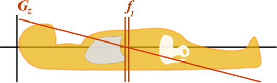
Let’s first just worry about the z-axis of your body, so imagine slicing up your body into little z-slices from your top of head to your toes. It would be great if we could cause just the protons in one of these little slices to precess, while we keep all of the other protons aligned with B0, because we would then be able to measure the T1 or T2 relaxation of the protons in just this slice. Well, we can do so by setting up B0 as a slice-selectiongradient,orGSS,that varies with location along the z-axis so that it is strongest at the top of your head and gradually gets weaker toward your feet, as shown in the picture below. Then, every slice along the z-axis will have a difference Larmor frequency, and we can use a RF pulse tuned to the specific Larmor frequency of the slice we want. In other words, our RF pulse can “select” the protons in a single slice along the z-axis of your body, like f1 in the picture, so that only those protons begin to precess. We call this process slice-selective excitation.
Remember, we’ve just selected a single slice– only the protons in that slice, and no other protons, are precessing. Since our readout relies completely on precession (because we can only measure changes in magnetic fields, as discussed in Part I), we’ve essentially isolated the signal from this slice, and we can now manipulate the protons in this slice to give us more information without affecting other protons– for example, we can now further isolate a single line of protons within the slice.
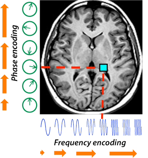
For this, we use a similar concept as before, but this time, we create a gradient in B0 in the y-direction, so that the magnetic field is strongest at your right ear and weakens toward your left ear, as shown in the picture below. Additionally, this time, we only turn on the gradient during readout, so that only the protons already precessing from slice-selection are affected. Since Larmor frequency depends upon B0, each line of protons from the right to the left of your body precess at a different speed. This localization technique is called frequency encoding, because this gradient encodes every line of protons within the slice with a different frequency depending on its location along the y-axis.
To measure the output from this, we use a math technique called a Fourier transform. You can read the intricacies of the math here, but essentially what you need to know is that combining waves with different characteristics and different frequencies creates a single wave with a unique structure. This also works in the reverse: we can to break down the composite wave into the waves that compose it. We pick up a single signal from all of the precessing protons, and using the Fourier transform, we can break down the signal into individuals signals from each line of protons.
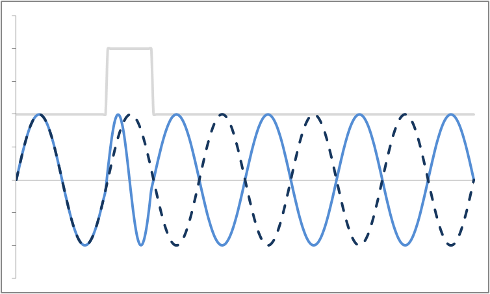
The last piece of the puzzle is that we can turn on a third phase-encoding gradient in B0 in the x-direction. In MRI, the phase-encoding gradient is turned on briefly and quickly switched off before we turn on the frequency-encoding gradient. As shown in the picture above, the brief phase-encoding gradient makes the protons at the front of your body precess more quickly than the protons at the back of your body. When it’s turned off, all of the protons return to their normal speed, but their rotations are slightly delayed from each other, creating a phase shift dependent on their location along the x-axis. In the picture below, the bump in the gray line represents the gradient turning on, and the dashed line represents the rotation of a proton near the back of your head, where the phase-encoding gradient is minimal. The light blue line represents the rotation of a proton near the front of your head– you can see that even though the two protons are precessing at the same frequency, there is a small time delay between their rotations.
So, just to summarize: All of MRI really revolves around this central idea of using magnetic fields to manipulate the magnetic fields inside your body in a way that can be measured and translated into an image. In an MRI, there’s a constant, large B0 from your head to your toes that lines up the protons in your body. We turn on a slice-selection gradient to “select” a single z-slice of your body by forcing the protons within that slice to precess. Then, we turn off this gradient and begin readout via the large current-measuring coils at the top of your head. During readout, we briefly turn on and switch off a phase-encoding gradient and then turn on a frequency-encoding gradient, effectively encoding every proton’s signal with its x- and y-position, which can be determined by its phase and frequency, respectively. (The loud sounds you hear inside an MRI are a result of all those gradients being turned on and off, which attract metals inside the machine and cause them to grate and strain against the other metals that hold them in place!) Lastly, we can parse out each proton’s signal by using a Fourier transform, and we can translate the signal to a single pixel in an MRI image, coloring it with a grayscale value that correlates to the T1 or T2 value of the tissue at that location in the body.
In our last post, we discussed the basic physics underlying magnetic resonance imaging, or MRI. But we haven’t built the complete picture yet– even with all of the physics that we talked about last time, we’re still only left with the ability to use a magnetic field to create a smaller magnetization vector inside the body that can then be measured by the electric current it induces in a loop of wire. How do we use this to create images of different types of tissue?
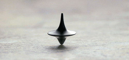
If you recall from our last post, we talked about the MRI producing an excess of spin up protons in your body, the magnetic moments of which sum to the measureable net magnetization vector, or NMV. To make this easier to visualize, let’s think of each excess spinning proton as a top, just like the mind-blowing eternally spinning one from Inception. As a result of the big magnetic field B0 pointing toward your head in the MRI, each of these little tops is lined up along B0 with its stem pointing toward your head and its tip toward your feet. Let’s also think of the magnetic moment produced by the spinning proton, which we can visualize as an arrow pointing along its axis of rotation, as essentially analogous to the top’s angular momentum– take a look at the arrow labeled L in the diagram below. In the absence of other forces, each proton acts just like a top set spinning with its stem perfectly vertical. It would keep spinning forever, precisely parallel to B0.
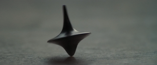
However, let’s say your top tips over just slightly, as it inevitably will in the real world– now the force of gravity isn’t perfectly aligned with the top’s axis of rotation. In fact, gravity now has a component perpendicular to the top’s angular momentum, as in the diagram above. This perpendicular component applies a torque that causes the top’s axis of rotation to rotate around its tip, changing the direction of the top’s spin without changing its speed. This phenomenon, called precession, is actually what you see in that wobbling circular motion of a top– see how its stem traces a circle, if viewed from bird’s-eye view?
We actually make use of precession for MRI. Remember how we said that the coil of wire at the head of the MRI can only measure changesin the z-component of the NVM? Well, we can change the z-components of our protons’ magnetic moments by making the protons precess. You see, when the magnetic moment is inclined so that it is no longer perfectly parallel to B0, its z-component shrinks. This is a simple matter of the Pythagorean theorem: try working it out to convince yourself that each leg of a triangle must be shorter than the hypotenuse. In fact, if we can get the proton to precess so that it is perpendicular to B0, its z-component will be 0.
We can cause precession by applying a little pulse of a magnetic force in the x- or y-direction, perpendicular to B0, to “pull” the proton’s magnetic moment (which lies along its axis of rotation) down and to the side. Let’s imagine we applied a little force to the right of the proton so that its magnetic moment tilts just a little to the right. Now, as its magnetic moment tilts forward and around to the left, we have to pull to the left in order to pull the magnetic moment further downward. So as the proton begins to precess, we have to apply an oscillating magnetic field, called a radiofrequency (RF) pulse, to pull its magnetic moment to the right as it rotates past the right, then left as it rotates past the left, then right again, left again, etc. in a swirl– all the while pulling it downward until it lies perpendicular to B0. This can be a little hard to visualize, so if you’re lost, try watching the first half of this video (until 0:03)!
For this RF pulse to be effective in rotating the proton’s magnetic moment to a desired angle, it has to come as close as possible to matching the frequency of the proton’s precession, which is called the Larmor frequency in MRI. If the RF pulse is out of sync with the Larmor frequency, it will be ineffective, kind of like pushing a swing at the wrong time. Now, a proton’s Larmor frequency depends on the strength of B0, the big magnetic field, at the specific location of the proton in question. This is a very important concept for what we’re going to be talking about in Part III, so keep this in mind!
After we use an RF pulse at the Larmor frequency of the proton long enough to force it to precess around the z-axis at a 90 degree angle, we just have to work out how to turn this precession into something measurable that we can use to differentiate between tissues. One way to do so is to use the density of protons, usually from water, in that tissue. Another way, which we’ll be discussing in further detail, is to use relaxation times, like T1 and T2.
At the beginning of the MRI, when we just have B0 without any other magnetic forces, our magnetization vector (which is, again, just a fancy name for the sum of the protons’ little magnetic moments) lies completely along the z-axis, so it has a really large z-component. Then, we use the RF pulse to force a 90 degree precession, so all of the protons precess in the XY-plane and the z-component of the magnetization vector decreases to a much smaller value. After we stop the RF pulse, however, these protons will gradually precess back to align with B0, essentially doing the opposite of the video above. As the protons do so, the NVM’s z-component exponentially increases back to its initial value. T1,orspin-lattice,relaxation measures the time constant of this recovery, marking the time at which approximately 63% of the original z-component. Because other atoms nearby can affect how easy it is for protons to precess back upward to align with B0, T1 varies between different types of tissues. Watch the second half of the video above (after 0:03) to see T1 in action.
In addition, when we apply the RF pulse to rotate the protons’ magnetic moments into the XY-plane, all of our protons precess in sync, with all of their magnetic moments aligned so that the magnetization vector oscillates between having a really large x-component and a really large y-component. As time passes, though, the protons dephase, getting out of sync with each other so that the x- and y-components of their magnetic moments cancel out. T2, or spin-spin,relaxation measures the time that it takes for the x- and y-components of the magnetization vector to decrease by 63%. This value also depends on the protons nearby, so T2, like T1, varies between tissues. You can see a bird’s eye view of T2dephasing in the video below, in which the translucent arrows represent individual magnetic moments, which sum to the big bright yellow arrow, or the magnetization vector.
Wow, that was a doozy. We zoomed in on individual protons, combining physics and math to figure out how to change their rotation to produce something that our wire coils can pick up and measure. In our next post, we just have to worry about the easy part– how to localize different tissues to specific locations in your body. Stay tuned!
Magnetic resonance imaging (MRI) seems like a crazy idea, when you think about it. How is it even possible to use magnets to create a 3D map of your body?
First, we have to understand something about the little tiny protons in the nuclei of the atoms that make up your body. If we’re to be very reductionist, we can think of protons as essentially “spinning” positive charges, and in physics, spinning charges produce magnetic fields that can then interact with other magnetic fields.
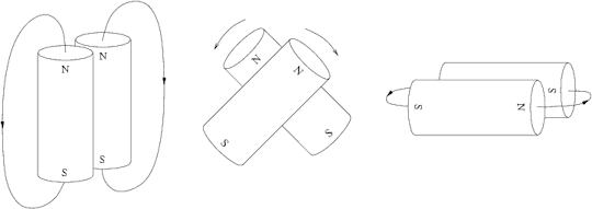
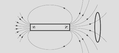
In fact, the interaction isn’t all that different from what you would intuit from playing with bar magnets as a kid. Let’s do a thought experiment– let’s say you had two bar magnets. How would you place it them so that, in the absence of external forces, neither one of them rotates due to the other’s magnetic field? Try it out, if you have a few magnets on hand, and see what you find!
Well, the obvious answer is that you can line them parallel to each other so that the poles on the first magnet align with the opposite poles on the other. The less obvious answer is that they can also be antiparallel to each other, so that both the North and South poles of the two magnets are lined up, as in the left panel of the diagram below. In this configuration, though, any little disturbance would cause the magnets to rotate and ultimately end up aligned in the first configuration, which is the most stable and energetically favored configuration.
In the absence of a big magnetic field, the spins of the protons in your body go in all kinds of directions so that the little magnetic fields they produce effectively cancel each other out. But when there IS a big external magnetic field, the protons’ magnetic fields take the two configurations we mentioned above in the thought experiments. We call the energetically favored parallel configuration spin up, and the other antiparallel configuration spin down.
Because spin up is energetically favored and more stable, there are always more spin up protons than spin down protons. These excess spin up protons produce a small but measurable magnetic moment called the net magnetization vector, or NMV,that lies parallel to the big magnetic field.
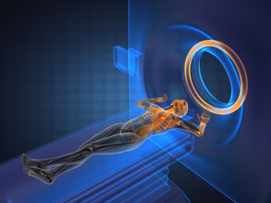
Imagine you’re lying on MRI table. Let’s map your body onto a 3D coordinate system, with the x-axis going from back to front, y-axis from left to right, and z-axis from bottom to top. MRI uses a big magnetic field along the z-axis of your body, going from your feet to the top of your head. We call this field B0, and it lines up the protons in your body to produce a NMV that also goes from your feet to your head.
Now, we just have to figure out how to measure this NMV. Actually, that’s what the big golden coil at the head of the patient in the illustration above is for. Remember when we said that spinning charges create magnetic fields? Well, it turns out that changing magnetic fields can also induce the movement of charges.
More accurately, changes in magnetic flux, or the number of magnetic field lines passing through a surface like the circle of space enclosed by the loop of wire in the diagram above, induce this movement of charge. Let’s imagine the NMV in your body as effectively a little bar magnet to the left of the wire loop. You see, this circle enclosed by the loop prefers to keep the number of magnetic field lines passing through it constant. If the the bar magnet were to hypothetically become stronger, more field lines would pass through the wire loop. Thus, the electric charges inside the wire would begin to flow in a way to produce a magnetic field inside the circle that counteracts the bar magnet’s effect on the flux. This phenomenon is called Lenz’s Law[1].
To put this all together, MRI uses a big magnetic field B0 to line up all the protons in your body to produce an NVM from your toes to your head. Whenever the z-component of your NMV inside the MRI system changes, it induces a current of a specific direction and strength within the coil at your head that can be easily measured.
So basically, even though you’re not normally a walking magnet, the MRI machine makes you into a tiny weak magnet, and then measures the strength and direction of your body’s magnetic fields to map you. Isn’t that awesome?
In Part II, we’ll talk about how to manipulate these basic concepts to map specific areas of your body. Stay tuned!
Cornell researchers get crafty in their paper published in August’s Nature.
A group at Cornell University has been playing with graphene and combining it with a technique called kirigami. Like origami, kirigami is Japanese paper folding, but with a twist– you can cut the paper in addition to folding it.
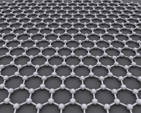
Graphene is an allotrope (form) of carbon, in which the carbon atoms are arranged into stacked single-atom thick layers of hexagons. This means you can get microscopic sheets of graphene– check out the picture above to see what a graphene sheet would look like at the atomic level! Graphene may prove very useful for scientists and engineers because it has electronic properties that may allow it to replace silicon in microchips. In order to build the graphene structures necessary for tiny nanodevices, however, scientists first needed to figure out how to manipulate graphene effectively. Noting that the mechanical behavior of the graphene was similar to that of regular old paper, the Cornell researchers decided to test the application of kirigami-inspired techniques to create their graphene structures.
The first step for the researchers was, naturally, to figure out how to move the graphene sheets. Although monolayer (single-atom) graphene sheets could be made through a process calledchemical vapor deposition, which can be thought of as “condensing” a vapor-like form of carbon onto the surface of a piece of copper, moving these microsheets around was a lot more difficult– graphene, at this thickness, very easily crumples and sticks permanently to itself. The researchers solved this problem by floating these graphene sheets in water with surfactants, which act like soap to make the sheets slippery and easier to handle.
The next step was to head to the Art Department to create full scale models of kirigami structures they wanted to build. After making the models, they began the process of building with graphene. To begin, graphene was bonded with aluminum, along with gold pads on either side of the graphene to limit direct contact from the researchers. Then, light was used to harden and strengthen only the graphene they wished to keep. Finally, unwanted graphene was removed with oxygen plasma and the aluminum removed with a weak acid. All in all, the process isn’t too much unlike its inspiration; just as kirigami requires you to trace along the patterns you want to keep with scissors and discard the pieces you cut out, working with graphene in this way is a subtractive form of manufacturing.
This allowed the team to create graphene springs and pyramid shapes that work as flexible transistors, which could become a key component in wearable electronics. It could also enhance personal technology, with the creation of folding tablets and TV screens. Medically, it could be used for comfortable heart sensors and medical devices for 24/7 use by at-risk patients. Additionally, the authors write that this graphene construction has potential to create sensors that respond to the tiniest amounts of force, improving detection. The Cornell researchers intend to pursue all avenues to find applications for this amazing new method.
While 2D printing, a process familiar to many, is used to draw images on a flat surface, 3D printing – also called additive manufacturing – is a process used to create three-dimensional objects. In additive processes, successive layers of materials are laid down under computer control until an entire object is created. This method of 3D printing has many applications, ranging from mass production of machine parts to building food models.
Initially, the digital 3D model is generated from a Computer Aided Design (CAD) program or a 3D scanner before printing software divides it into very small horizontal layers and uploads it into the printer, which proceeds to create each layer one at a time, blending them together so that no signs of the layering remain visible. A wide range of materials can be used for 3D printing, including plastic, glass, metal, wax, even edible food.
To summarize, 3D printing can be done in different ways depending on the purpose, number of items, materials used, and complexity of the objects. For more information about 3D printing, click here.


![https://commons.wikimedia.org/wiki/File:Graphen.jpg#/media/File:Graphen.jpg]](https://commons.wikimedia.org/wiki/File:Graphen.jpg#/media/File:Graphen.jpg%5D)

