Previously in this blog a number of attempts have been made to explicate the Taoist number line and contrast it with the Western version of the same. It is essential to do this and to do it flawlessly, first because different systems of arithmetic result from the two, and secondly because the mandalic coordinate system is based on the former perspective while the Cartesian coordinate system is based on the latter.[1]
What has been offered earlier has been accurate to a degree, a good first approximation. Here we intend to present a more definitive account of the Taoist number line, describing both how it is similar to and how it differs from the Western number line used by Descartes in formation of his coordinate system. This will inevitably transport us well beyond that comfort zone offered by the more accessible three-dimensional cubic box that has heretofore engaged us.
Both Taoist and Western number lines observe directional locative division of their single dimension into two major partitions: positive and negative for the West; yinandyang for Taoism.[2] There the similarities essentially end. From its earliest beginnings Taoism recognized a second directional divisioning in its number line, that of manifest/unmanifestorbeingandbecoming.[3] The West never did such. As a result, some time later the West found it necessary to invent imaginary numbers.[4][5]
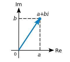
Descartes knew of these numbers but was not particularly fond of them. It was he, in fact, who first used the term “imaginary” describing them in a derogatory sense. [Wikipedia] The term “imaginary number” now just denotes a complex number with a real part equal to 0, that is, a number of the form bi. A complex number where the real part is other than 0 is represented by the form a + bi.
In place of the complex plane, Taoism has (and always has had from time immemorial) a plane of potentiality. An explanation of this alternative plane was attempted earlier in this blog, but it can likely be improved. This post has simply been a broad brushstrokes overview. In the following posts we will look more closely at the specifics involved.[6]
Image (lower): A complex number can be visually represented as a pair of numbers (a, b) forming a vector on a diagram representing the complex plane. “Re” is the real axis, “Im” is the imaginary axis, and i is the imaginary unit which satisfies i2 = −1. Wolfkeeper at English Wikipedia [GFDL (http://www.gnu.org/copyleft/fdl.html) or CC BY-SA 3.0 (http://creativecommons.org/licenses/by-sa/3.0)], via Wikimedia Commons
Notes
[1] The arithmetic system derived from the Taoist number line can perhaps best be understood as a noumenal one. It applies to the world of ideas rather than to our phenomenal world of the physical senses, but it may also apply to the real world, that is, the real real world which we can never fully access.
Much of modern philosophy has generally been skeptical of the possibility of knowledge independent of the physical senses, and Immanuel Kant gave this point of view its canonical expression: that the noumenal world may exist, but it is completely unknowable to humans. In Kantian philosophy, the unknowable noumenon is often linked to the unknowable “thing-in-itself” (Ding an sich, which could also be rendered as “thing as such” or “thing per se”), although how to characterize the nature of the relationship is a question yet open to some controversy. [Wikipedia]
[2] From the perspective of physics this involves a division into two major quanta of charge, negative and positive, which like yinandyang can be either complementary or opposing. Like forces repel one another and unlike attract. This is the basis of electromagnetism, one of four forces of nature recognized by modern physics. But it is likely also the basis, though not fully recognized as such, of the strong and weak nuclear forces, possibly of the force of gravity as well. I would suspect that to be the case. The significant differences among the forces (or force fields, the term physics now prefers to use) lie mainly, as we shall see, in intricate twistings and turnings through various dimensions or directions that negative and positive charges undergo in particle interactions.
[3] It is this additional axis of probabilistic directional location, along with composite dimensioning, both of which are unique to mandalic geometry, that make it a geometry of spacetime, in contrast to Descartes’ geometry which, in and of itself, is one of space alone. The inherent spatiotemporal dynamism that is characteristic of mandalic coordinates makes them altogether more relevant for descriptions of particle interactions than Cartesian coordinates, which often demand complicated external mathematical mechanisms to sufficiently enliven them to play even a partial descriptive role, however inadequate.
[4] In addition to their use in mathematics, complex numbers, once thought to be "fictitious" and useless, have found practical applications in many fields, including chemistry, biology, electrical engineering, statistics, economics, and, most importantly perhaps, physics..
[5] The Italian mathematician Gerolamo Cardano is the first known to have introduced complex numbers. He called them “fictitious” during his attempts to find solutions to cubic equations in the 16th century. At the time, such numbers were poorly understood, consequently regarded by many as fictitious or useless as negative numbers and zero once were. Many other mathematicians were slow to adopt use of imaginary numbers, including Descartes, who referred to them in his La Géométrie, in which he introduced the term imaginary, that was intended to be derogatory. Imaginary numbers were not widely accepted until the work of Leonhard Euler (1707–1783) and Carl Friedrich Gauss (1777–1855). Geometric interpretation of complex numbers as points in a complex plane was first stated by mathematician and cartographer Caspar Wessel in 1799. [Wikipedia]
[6] What I have called here the plane of potentiality occurs only implicitly in the Taoist I Ching but is fully developed in mandalic geometry. It may be related to bicomplex numbers or tessarines in abstract algebra, the existence of which I only just discovered. Unlike the quaternions first described by Hamilton in 1843, which extended the complex plane to three dimensions, but unfortunately are not commutative, tesserines or bicomplex numbers are hypercomplex numbers in a commutative, associative algebra over real numbers, with two imaginary units (designated i and k). Reading further, I find the following fascinating remark,
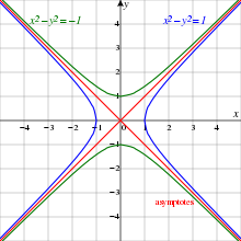
The rectangular hyperbola x2-y2 and its conjugate, having the same asymptotes. The Unit Hyperbola is blue, its conjugate is green, and the asymptotes are red. By Own work (Based on File:Drini-conjugatehyperbolas.png) [CC BY-SA 2.5],via Wikimedia Commons
Note to self: Also investigate Cayley–Dickson constructionandzero divisor. Remember, this is a work still in progress, and if a bona fide mathematician believes division by zero is possible in some circumstances, (as is avowed by mandalic geometry), I want to find out more about it.
Please note: The content and/or format of this post may not be in finalized form. Reblog as a TEXT post will contain this caveat alerting readers to refer to the current version in the source blog. A LINK post will itself do the same. :)
Scroll to bottom for links to Previous / Next pages (if existent). This blog builds on what came before so the best way to follow it is chronologically. Tumblr doesn’t make that easy to do. Since the most recent page is reckoned as Page 1 the number of the actual Page 1 continually changes as new posts are added. To determine the number currently needed to locate Page 1 go to the most recent post which is here. The current total number of pages in the blog will be found at the bottom. The true Page 1 can be reached by changing the web address mandalicgeometry.tumblr.com to mandalicgeometry.tumblr.com/page/x, exchanging my current page number for x and entering. To find a different true page(p) subtract p from x+1 to get the number(n) to use. Place n in the URL instead of x (mandalicgeometry.tumblr.com/page/n) where n = x + 1 - p. :)
Dark Energy May Be Incompatible With String Theory
A controversial new paper argues that universes with dark energy profiles like ours do not exist in the “landscape” of universes allowed by string theory.
On June 25, Timm Wrase awoke in Vienna and groggily scrolled through an online repository of newly posted physics papers. One title startled him into full consciousness.
Thepaper, by the prominent string theorist Cumrun Vafa of Harvard University and collaborators, conjectured a simple formula dictating which kinds of universes are allowed to exist and which are forbidden, according to string theory. The leading candidate for a “theory of everything” weaving the force of gravity together with quantum physics, string theory defines all matter and forces as vibrations of tiny strands of energy. The theory permits some 10500 different solutions: a vast, varied “landscape” of possible universes. String theorists like Wrase and Vafa have strived for years to place our particular universe somewhere in this landscape of possibilities.
But now, Vafa and his colleagues were conjecturing that in the string landscape, universes like ours — or what ours is thought to be like — don’t exist. If the conjecture is correct, Wrase and other string theorists immediately realized, the cosmos must either be profoundly different than previously supposed or string theory must be wrong.
After dropping his kindergartner off that morning, Wrase went to work at the Vienna University of Technology, where his colleagues were also buzzing about the paper. That same day, in Okinawa, Japan, Vafa presented the conjecture at the Strings 2018 conference, which was streamed by physicists worldwide. Debate broke out on- and off-site. “There were people who immediately said, ‘This has to be wrong,’ other people who said, ‘Oh, I’ve been saying this for years,’ and everything in the middle,” Wrase said. There was confusion, he added, but “also, of course, huge excitement. Because if this conjecture was right, then it has a lot of tremendous implications for cosmology.”
Researchers have set to work trying to test the conjecture and explore its implications. Wrase has already written two papers, including one that may lead to a refinement of the conjecture, and both mostly while on vacation with his family. He recalled thinking, “This is so exciting. I have to work and study that further.”
The conjectured formula — posed in the June 25 paper by Vafa, Georges Obied, Hirosi Ooguri and Lev Spodyneiko and further explored in a second paper released two days later by Vafa, Obied, Prateek Agrawal and Paul Steinhardt — says, simply, that as the universe expands, the density of energy in the vacuum of empty space must decrease faster than a certain rate. The rule appears to be true in all simple string theory-based models of universes. But it violates two widespread beliefs about the actual universe: It deems impossible both the accepted picture of the universe’s present-day expansion and the leading model of its explosive birth.
Dark Energy in Question
Since 1998, telescope observations have indicated that the cosmos is expanding ever-so-slightly faster all the time, implying that the vacuum of empty space must be infused with a dose of gravitationally repulsive “dark energy.”
But the new conjecture asserts that the vacuum energy of the universe must be decreasing.
Vafa and colleagues contend that universes with stable, constant, positive amounts of vacuum energy, known as “de Sitter universes,” aren’t possible. String theorists have struggled mightily since dark energy’s 1998 discovery to construct convincing stringy models of stable de Sitter universes. But if Vafa is right, such efforts are bound to sink in logical inconsistency; de Sitter universes lie not in the landscape, but in the “swampland.” “The things that look consistent but ultimately are not consistent, I call them swampland,” he explained recently. “They almost look like landscape; you can be fooled by them. You think you should be able to construct them, but you cannot.”
According to this “de Sitter swampland conjecture,” in all possible, logical universes, the vacuum energy must either be dropping, its value like a ball rolling down a hill, or it must have obtained a stable negative value. (So-called “anti-de Sitter” universes, with stable, negative doses of vacuum energy, are easily constructed in string theory.)
The conjecture, if true, would mean the density of dark energy in our universe cannot be constant, but must instead take a form called “quintessence” — an energy source that will gradually diminish over tens of billions of years. Several telescope experiments are underway now to more precisely probe whether the universe is expanding with a constant rate of acceleration, which would mean that as new space is created, a proportionate amount of new dark energy arises with it, or whether the cosmic acceleration is gradually changing, as in quintessence models. A discovery of quintessence would revolutionize fundamental physics and cosmology, including rewriting the cosmos’s history and future. Instead of tearing apart in a Big Rip, a quintessent universe would gradually decelerate, and in most models, would eventually stop expanding and contract in either a Big Crunch or Big Bounce.
Paul Steinhardt, a cosmologist at Princeton University and one of Vafa’s co-authors, said that over the next few years, “all eyes should be on” measurements by the Dark Energy Survey, WFIRST and Euclid telescopes of whether the density of dark energy is changing. “If you find it’s not consistent with quintessence,” Steinhardt said, “it means either the swampland idea is wrong, or string theory is wrong, or both are wrong or — something’s wrong.”
Inflation Under Siege
No less dramatically, the new swampland conjecture also casts doubt on the widely believed story of the universe’s birth: the Big Bang theory known as cosmic inflation. According to this theory, a minuscule, energy-infused speck of space-time rapidly inflated to form the macroscopic universe we inhabit. The theory was devised to explain, in part, how the universe got so huge, smooth and flat.
But the hypothetical “inflaton field” of energy that supposedly drove cosmic inflation doesn’t sit well with Vafa’s formula. To abide by the formula, the inflaton field’s energy would probably have needed to diminish too quickly to form a smooth- and flat-enough universe, he and other researchers explained. Thus, the conjecture disfavors many popular models of cosmic inflation. In the coming years, telescopes such as the Simons Observatory will look for definitive signatures of cosmic inflation, testing it against rival ideas.
In the meantime, string theorists, who normally form a united front, will disagree about the conjecture. Eva Silverstein, a physics professor at Stanford University and a leader in the effort to construct string-theoretic models of inflation, thinks it is very likely to be false. So does her husband, the Stanford professor Shamit Kachru; he is the first “K” in KKLT, a famous 2003 paper (known by its authors’ initials) that suggested a set of stringy ingredients that might be used to construct de Sitter universes. Vafa’s formula says both Silverstein’s and Kachru’s constructions won’t work. “We’re besieged by these conjectures in our family,” Silverstein joked. But in her view, accelerating-expansion models are no more disfavored now, in light of the new papers, than before. “They essentially just speculate that those things don’t exist, citing very limited and in some cases highly dubious analyses,” she said.
Matthew Kleban, a string theorist and cosmologist at New York University, also works on stringy models of inflation. He stresses that the new swampland conjecture is highly speculative and an example of “lamppost reasoning,” since much of the string landscape has yet to be explored. And yet he acknowledges that, based on existing evidence, the conjecture could well be true. “It could be true about string theory, and then maybe string theory doesn’t describe the world,” Kleban said. “[Maybe] dark energy has falsified it. That obviously would be very interesting.”
Mapping the Swampland
Whether the de Sitter swampland conjecture and future experiments really have the power to falsify string theory remains to be seen. The discovery in the early 2000s that string theory has something like 10500 solutions killed the dream that it might uniquely and inevitably predict the properties of our one universe. The theory seemed like it could support almost any observations and became very difficult to experimentally test or disprove.
In 2005, Vafa and a network of collaborators began to think about how to pare the possibilities down by mapping out fundamental features of nature that absolutely have to be true. For example, their “weak gravity conjecture” asserts that gravity must always be the weakest force in any logical universe. Imagined universes that don’t satisfy such requirements get tossed from the landscape into the swampland. Many of these swampland conjectures have held up famously against attack, and some are now “on a very solid theoretical footing,” said Hirosi Ooguri, a theoretical physicist at the California Institute of Technology and one of Vafa’s first swampland collaborators. The weak gravity conjecture, for instance, has accumulated so much evidencethat it’s now suspected to hold generally, independent of whether string theory is the correct theory of quantum gravity.
The intuition about where landscape ends and swampland begins derives from decades of effort to construct stringy models of universes. The chief challenge of that project has been that string theory predicts the existence of 10 space-time dimensions — far more than are apparent in our 4-D universe. String theorists posit that the six extra spatial dimensions must be small — curled up tightly at every point. The landscape springs from all the different ways of configuring these extra dimensions. But although the possibilities are enormous, researchers like Vafa have found that general principles emerge. For instance, the curled-up dimensions typically want to gravitationally contract inward, whereas fields like electromagnetic fields tend to push everything apart. And in simple, stable configurations, these effects balance out by having negative vacuum energy, producing anti-de Sitter universes. Turning the vacuum energy positive is hard. “Usually in physics, we have simple examples of general phenomena,” Vafa said. “De Sitter is not such a thing.”
The KKLT paper, by Kachru, Renata Kallosh, Andrei Linde and Sandip Trivedi, suggested stringy trappings like “fluxes,” “instantons” and “anti-D-branes” that could potentially serve as tools for configuring a positive, constant vacuum energy. However, these constructions are complicated, and over the years possible instabilities have been identified. Though Kachru said he does not have “any serious doubts,” many researchers have come to suspect the KKLT scenario does not produce stable de Sitter universes after all.
Vafa thinks a concerted search for definitely stable de Sitter universe models is long overdue. His conjecture is, above all, intended to press the issue. In his view, string theorists have not felt sufficiently motivated to figure out whether string theory really is capable of describing our world, instead taking the attitude that because the string landscape is huge, there must be a place in it for us, even if no one knows where. “The bulk of the community in string theory still sides on the side of de Sitter constructions [existing],” he said, “because the belief is, ‘Look, we live in a de Sitter universe with positive energy; therefore we better have examples of that type.’”
His conjecture has roused the community to action, with researchers like Wrase looking for stable de Sitter counterexamples, while others toy with little-explored stringy models of quintessent universes. “I would be equally interested to know if the conjecture is true or false,” Vafa said. “Raising the question is what we should be doing. And finding evidence for or against it — that’s how we make progress.”
Mathematicians Disprove Conjecture Made to Save Black Holes
Mathematicians have disproved the strong cosmic censorship conjecture. Their work answers one of the most important questions in the study of general relativity and changes the way we think about spacetime.
Nearly 40 years after it was proposed, mathematicians have settled one of the most profound questions in the study of general relativity. In a paper posted online last fall, mathematicians Mihalis DafermosandJonathan Luk have proven that the strong cosmic censorship conjecture, which concerns the strange inner workings of black holes, is false.
“I personally view this work as a tremendous achievement — a qualitative jump in our understanding of general relativity,” emailed Igor Rodnianski, a mathematician at Princeton University.
The strong cosmic censorship conjecture was proposed in 1979 by the influential physicist Roger Penrose. It was meant as a way out of a trap. For decades, Albert Einstein’s theory of general relativity had reigned as the best scientific description of large-scale phenomena in the universe. Yet mathematical advances in the 1960s showed that Einstein’s equations lapsed into troubling inconsistencies when applied to black holes. Penrose believed that if his strong cosmic censorship conjecture were true, this lack of predictability could be disregarded as a mathematical novelty rather than as a sincere statement about the physical world.
“Penrose came up with a conjecture that basically tried to wish this bad behavior away,” said Dafermos, a mathematician at Princeton University.
This new work dashes Penrose’s dream. At the same time, it fulfills his ambition by other means, showing that his intuition about the physics inside black holes was correct, just not for the reason he suspected.
Relativity’s Cardinal Sin
In classical physics, the universe is predictable: If you know the laws that govern a physical system and you know its initial state, you should be able to track its evolution indefinitely far into the future. The dictum holds true whether you’re using Newton’s laws to predict the future position of a billiard ball, Maxwell’s equations to describe an electromagnetic field, or Einstein’s theory of general relativity to predict the evolution of the shape of space-time. “This is the basic principle of all classical physics going back to Newtonian mechanics,” said Demetrios Christodoulou, a mathematician at ETH Zurich and a leading figure in the study of Einstein’s equations. “You can determine evolution from initial data.”
But in the 1960s mathematicians found a physical scenario in which Einstein’s field equations — which form the core of his theory of general relativity — cease to describe a predictable universe. Mathematicians and physicists noticed that something went wrong when they modeled the evolution of space-time inside a rotating black hole.
To understand what went wrong, imagine falling into the black hole yourself. First you cross the event horizon, the point of no return (though to you it looks just like ordinary space). Here Einstein’s equations still work as they should, providing a single, deterministic forecast for how space-time will evolve into the future.
But as you continue to travel into the black hole, eventually you pass another horizon, known as the Cauchy horizon. Here things get screwy. Einstein’s equations start to report that many different configurations of space-time could unfold. They’re all different, yet they all satisfy the equations. The theory cannot tell us which option is true. For a physical theory, it’s a cardinal sin.
“The loss of predictability that we seem to find in general relativity was very disturbing,” said Eric Poisson, a physicist at the University of Guelph in Canada.
Roger Penrose proposed the strong cosmic censorship conjecture to restore predictability to Einstein’s equations. The conjecture says that the Cauchy horizon is a figment of mathematical thought. It might exist in an idealized scenario where the universe contains nothing but a single rotating black hole, but it can’t exist in any real sense.
The reason, Penrose argued, is that the Cauchy horizon is unstable. He said that any passing gravitational waves should collapse the Cauchy horizon into a singularity — a region of infinite density that rips space-time apart. Because the actual universe is rippled with these waves, a Cauchy horizon should never occur in the wild.
As a result, it’s nonsensical to ask what happens to space-time beyond the Cauchy horizon because space-time, as it’s regarded within the theory of general relativity, no longer exists. “This gives one a way out of this philosophical conundrum,” said Dafermos.
This new work shows, however, that the boundary of space-time established at the Cauchy horizon is less singular than Penrose had imagined.
To Save a Black Hole
Dafermos and Luk, a mathematician at Stanford University, proved that the situation at the Cauchy horizon is not quite so simple. Their work is subtle — a refutation of Penrose’s original statement of the strong cosmic censorship conjecture, but not a complete denial of its spirit.
Building on methods established a decade ago by Christodoulou, who was Dafermos’s adviser in graduate school, the pair showed that the Cauchy horizon can indeed form a singularity, but not the kind Penrose anticipated. The singularity in Dafermos and Luk’s work is milder than Penrose’s — they find a weak “light-like” singularity where he had expected a strong “space-like” singularity. This weaker form of singularity exerts a pull on the fabric of space-time but doesn’t sunder it. “Our theorem implies that observers crossing the Cauchy horizon are not torn apart by tidal forces. They may feel a pinch, but they are not torn apart,” said Dafermos in an email.
Because the singularity that forms at the Cauchy horizon is in fact milder than predicted by the strong cosmic censorship conjecture, the theory of general relativity is not immediately excused from considering what happens inside. “It still makes sense to define the Cauchy horizon because one can, if one wishes, continuously extend the space-time beyond it,” said Harvey Reall, a physicist at the University of Cambridge.
Dafermos and Luk prove that space-time extends beyond the Cauchy horizon. They also prove that from the same starting point, it can extend in any number of ways: Past the horizon “there are many such extensions that one could entertain, and there is no good reason to prefer one to the other,” said Dafermos.
Yet — and here’s the subtlety in their work — these nonunique extensions of space-time don’t mean that Einstein’s equations go haywire beyond the horizon.
Why Is M-Theory the Leading Candidate for Theory of Everything?
The mother of all string theories passes a litmus test that, so far, no other candidate theory of quantum gravity has been able to match.
It’s not easy being a “theory of everything.” A TOE has the very tough job of fitting gravity into the quantum laws of nature in such a way that, on large scales, gravity looks like curves in the fabric of space-time, as Albert Einstein described in his general theory of relativity. Somehow, space-time curvature emerges as the collective effect of quantized units of gravitational energy — particles known as gravitons. But naive attempts to calculate how gravitons interact result in nonsensical infinities, indicating the need for a deeper understanding of gravity.
String theory (or, more technically, M-theory) is often described as the leading candidate for the theory of everything in our universe. But there’s no empirical evidence for it, or for any alternative ideas about how gravity might unify with the rest of the fundamental forces. Why, then, is string/M-theory given the edge over the others?
The theory famously posits that gravitons, as well as electrons, photons and everything else, are not point-particles but rather imperceptibly tiny ribbons of energy, or “strings,” that vibrate in different ways. Interest in string theory soared in the mid-1980s, when physicists realized that it gave mathematically consistent descriptions of quantized gravity. But the five known versions of string theory were all “perturbative,” meaning they broke down in some regimes. Theorists could calculate what happens when two graviton strings collide at high energies, but not when there’s a confluence of gravitons extreme enough to form a black hole.
Then, in 1995, the physicist Edward Witten discovered the mother of all string theories. He found various indications that the perturbative string theories fit together into a coherent nonperturbative theory, which he dubbed M-theory. M-theory looks like each of the string theories in different physical contexts but does not itself have limits on its regime of validity — a major requirement for the theory of everything. Or so Witten’s calculations suggested. “Witten could make these arguments without writing down the equations of M-theory, which is impressive but left many questions unanswered,” explained David Simmons-Duffin, a theoretical physicist at the California Institute of Technology.
Another research explosion ensued two years later, when the physicist Juan Maldacenadiscovered the AdS/CFT correspondence: a hologram-like relationship connecting gravity in a space-time region called anti-de Sitter (AdS) space to a quantum description of particles (called a “conformal field theory”) moving around on that region’s boundary. AdS/CFT gives a complete definition of M-theory for the special case of AdS space-time geometries, which are infused with negative energy that makes them bend in a different way than our universe does. For such imaginary worlds, physicists can describe processes at all energies, including, in principle, black hole formation and evaporation. The 16,000 papers that have cited Maldacena’s over the past 20 years mostly aim at carrying out these calculations in order to gain a better understanding of AdS/CFT and quantum gravity.
This basic sequence of events has led most experts to consider M-theory the leading TOE candidate, even as its exact definition in a universe like ours remains unknown. Whether the theory is correct is an altogether separate question. The strings it posits — as well as extra, curled-up spatial dimensions that these strings supposedly wiggle around in — are 10 million billion times smaller than experiments like the Large Hadron Collider can resolve. And some macroscopic signatures of the theory that might have been seen, such as cosmic strings and supersymmetry, have not shown up.
Other TOE ideas, meanwhile, are seen as having a variety of technical problems, and none have yet repeated string theory’s demonstrations of mathematical consistency, such as the graviton-graviton scattering calculation. (According to Simmons-Duffin, none of the competitors have managed to complete the first step, or first “quantum correction,” of this calculation.) One philosopher has even argued that string theory’s status as the only known consistent theory counts as evidence that the theory is correct.
The distant competitors include asymptotically safe gravity,E8 theory,noncommutative geometryandcausal fermion systems. Asymptotically safe gravity, for instance, suggests that the strength of gravity might change as you go to smaller scales in such a way as to cure the infinity-plagued calculations. But no one has yet gotten the trick to work.
“..I had two passions when I was a child. First was to learn about Einstein’s theory and help to complete his dream of a unified theory of everything. That’s my day job. I work in something called string theory. I’m one of the founders of the subject. We hope to complete Einstein’s dream of a theory of everything..”
― Theoretical physicist Michio Kaku (Co-founder of string field theory)
This post is going to try and explain the concepts of Lagrangian mechanics, with minimal derivations and mathematical notation. By the end of it, hopefully you will know what my URL is all about.
Some mechanicses which happened in the past
In 1687, Isaac Newton became the famousest scientist jerk in Europe by writing a book called Philosophiæ Naturalis Principia Mathematica. The book gave a framework of describing motion of objects that worked just as well for stuff in space as objects on the ground. Physicists spent the next couple of hundred years figuring out all the different things it could be applied to.
(Newton’s mechanics eventually got downgraded to ‘merely a very good approximation’ when quantum mechanics and relativity came along to complicate things in the 1900s.)
In 1788, Joseph-Louise Lagrange found a different way to put Newton’s mechanics together, using some mathematical machinery called Calculus of Variations. This turned out to be a very useful way to look at mechanics, almost always much easier to operate, and also, like, the basis for all theoretical physics today.
We call this Lagrangian mechanics.
What’s the point of a mechanics?
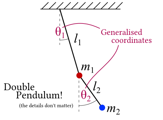
The way we think of it these days is, whatever we’re trying to describe is a physical system. For example, this cool double pendulum.
The physical system has a state - “the pieces of the system are arranged this way”. We can describe the state with a list of numbers. The double pendulum might use the angles of the two pendulums. The name for these numbers, in Lagrangian mechanics, is generalised coordinates.
(Why are they “generalised”? When Newton did his mechanics to begin with, everything was thought of as ‘particles’ with a position in 3D space. The coordinates are each particle’s \(x\), \(y\) and \(z\) position. Lagrangian mechanics, on the other hand is cool with any list of numbers can be used to distinguish the different states of the system, so its coordinates are “generalised”.)
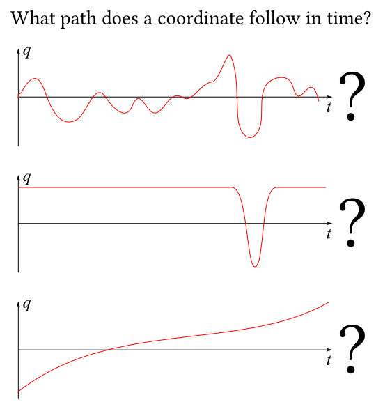
Now, we want to know what the system does as time advances. This amounts to knowing the state of the system for every single point in time.
There are lots of possibilities for what a system might do. The double pendulum might swing up and hold itself horizontal forever, for example, or spin wildly. We call each one a path.
Because the generalised coordinates tell apart all the different states of the system, a path amounts to a value of each generalised coordinate at every point in time.
OK. The point of mechanics is to find out which of the many imaginable paths the system/each coordinate actuallytakes.
The Action
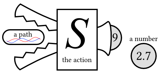
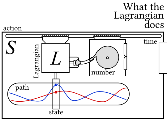
To achieve this, Lagrangian mechanics says the system has a mathematical object associated with it called the action. It’s almost always written as \(S\).
OK, so here’s what you do with the action: you take one of the paths that the system might take, and feed it in; the action then spits out a number. (It’s an object called a functional, to mathematicans: a function from functions to numbers).
So every path the system takes gets a number associated with it by the action.
The actual numbers associated with each path are not actually that useful. Rather, we want to compare ‘nearby’ paths.
We’re looking for a path with a special property: if you add any tiny little extra wiggle to the path, and feed the new path through the action, you get the same number out. We say that the path with this special property is the one the system actually takes.
This is called the principle of stationary action. (It’s sometimes called the “principle of least action”, but since the path we’re interested in is not necessarily the path for which the action is lowest, you shouldn’t call it that.)
But why does it do that
The answer is sort of, because we pick out an action which produces a stationary path corresponding to our system. Which might sound rather circular and pointless.
If you study quantum field theory, you find out the principle of stationary action falls out rather neatly from a calculation called the Path Integral. So you could say that’s “why”, but then you have the question of “why quantum field theory”.
A clearer question is why is it useful to invent an object called the action that does this thing. A couple of reasons:
the general properties actions frequently make it possible to work out the action of a system just by looking at it, and it’s easier to calculate things this way than the Newtonian way.
the action gives us a mathematical object that can be thought of as a ‘complete description of the behaviour of the system’, and conclusions you draw about this object - to do with things like symmetries and conserved quantities, say - are applicable to the system as well.
The Lagrangian
So, OK, let’s crack the action open and look at how it’s made up.
So “inside the action” there’s another object called the Lagrangian, usually written \(L\). (As far as I know it got called that by Hamilton, who was a big fan of Lagrange.) The Lagrangian takes a state of the system and a measure of how quickly its changing, and gives you back a number.
The action crawls along the path of the system, applying the Lagrangian at every point in time, and adding up all the numbers.
Mathematically, the action is the integral of the Lagrangian with respect to time. We write that like $$S[q]=\int_{q(t)} L(q,\dot{q},t)\dif t$$
What can you do with a Lagrangian?
Lots and lots of things.
The main thing is that you use the Lagrangian to figure out what the stationary path is.
Using a field of maths called calculus of variations, you can show that the path that stationaryises the action can be found from the Lagrangian by solving a set of differential equations called the Euler-Langrange equations. If you’re curious, they look like $$\frac{\dif}{\dif t}\left(\frac{\partial L}{\partial \dot{q}_i}\right) = \frac{\partial L}{\partial q_i}$$but we won’t go into the details of how they’re derived in this post.
The Euler-Lagrange equations give you the equations of motion of the system. (Newtonian mechanics would also give you the same equations of motion, eventually. From that point on - solving the equations of motion - everything is the same in all your mechanicses).
The Lagrangian has some useful properties. Constraints can be handled easily using the method of Lagrange multipliers, and you can add Lagrangians for components together to get the Lagrangian of a system with multiple parts.
These properties (and probably some others that I’m forgetting) tell us what a Lagrangian made of multiple Newtonian particles looks like, if we know the Lagrangian for a single particle.
Particles and Potentials (the new RPG!)
In the old, Newtonian mechanics, the world is made up of particles, which have a position in space, a number called a mass, and not much else. To determine the particles’ motion, we apply things called forces, which we add up and divide by the mass to give the acceleration of the particle.
Forces have a direction (they’re objects called vectors), and can depend on any number of things, but very commonly they depend on the particle’s position in space. You can have a field which associates a force (number and direction) with every single point in space.
Sometimes, forces have a special property of being conservative. A conservative force has the special property that
depends on where the particle is, but not how fast its going
if you move the particle in a loop, and add up the force times the distance moved at every point around the loop, you get zero
This is great, because now your force can be found from a potential. Instead of associating a vector with every point, the potential is a scalar field which just has a number (no direction) at each point.
This is great for lots of reasons (you can’t get very far in orbital mechanics or electromagnetism without potentials) but for our purposes, it’s handy because we might be able to use it in the Lagrangian.
How Lagrangians are made
So, suppose our particle can travel along a line. The state of the system can be described with only one generalised coordinate - let’s call it \(q(t)\). It’s being acted on by a conservative force, with a potential defined along the line which gives the force on the particle.
With this super simple system, the Lagrangian splits into two parts. One of them is $$T=\frac{1}{2}m\dot{q}^2$$which is a quantity which Newtonian mechanics calls the kinetic energy (but we’ll get to energy in a bit!), and the other is just the potential \(V(q)\). With these, the Lagrangian looks like $$L=T-V$$and the equations of motion you get are $$m\ddot{q}=-\frac{\dif V}{\dif q}$$exactly the same as Newtonian mechanics.
As it turns out, you can use that idea really generally. When things get relativistic (such as in electromagnetism), it gets squirlier, but if you’re just dealing with rigid bodies acting under gravity and similar situations? \(L=T-V\) is all you need.
This is useful because it’s usually a lot easier to work out the kinetic and potential energy of the objects in a situation, then do some differentiation, than to work out the forces on each one. Plus, constraints.
The Canonical Momentum
The canonical momentum in of itself isn’t all that interesting, actually! Though you use it to make Hamiltonian mechanics, and it hints towards Noether’s theorem, so let’s talk about it.
So the Lagrangian depends on the state of the system, and how quickly its changing. To be more specific, for each generalised coordinate \(q_i\), you have a ‘generalised velocity’ \(\dot{q}_i\) measuring how quickly it is changing in time at this instant. So for example at one particular instant in the double pendulum, one of the angles might be 30 degrees, and the corresponding velocity might be 10 radians per second.
Thecanonical momenta \(p_i\) can be thought of as a measure of how responsive the Lagrangian is to changes in the generalised velocity. Mathematically, it’s the partial differential (keeping time and all the other generalised coordinates and momenta stationary): $$p_i=\frac{\partial L}{\partial \dot{q}_i}$$They’re called momenta by analogy with the quantities linear momentumandangular momentum in Newtonian mechanics. For the example of the particle travelling in a conservative force, the canonical momentum is exactly the same as the linear momentum: \(p=m\dot{q}\). And for a rotating body, the canonical momentum is the same as the angular momentum. For a system of particles, the canonical momentum is the sum of the linear momenta.
But be careful! In situations like motion in a magnetic field, the canonical momentum and the linear momentum are different. Which has apparently led to no end of confusion for Actual Physicists with a problem involving a lattice and an electron and somethingorother I can no long remember…
OK a little maths; let’s grab the Euler-Lagrange equations again: $$\frac{\dif}{\dif t} \left(\frac{\partial L}{\partial \dot{q}}\right) = \frac{\partial L}{\partial q_i}$$Hold on. That’s the canonical momentum on the left. So we can write this as $$\frac{\dif p_i}{\dif t} = \frac{\partial L}{\partial q_i}$$Which has an interesting implication: suppose \(L\) does not depend on a coordinate directly, but only its velocity. In that case, the equation becomes $$\frac{\dif p_i}{\dif t}=0$$so the canonical momentum corresponding to this coordinate does not change ever, no matter what.
Which is known in Newtonian mechanics as conservation of momentum. So Lagrangian mechanics shows that momentum being conserved is equivalent to the Lagrangian not depending on the absolute positions of the particles…
That’s a special case of a very very important theorem invented by Emmy Noether.
The canonical momenta (or in general, the canonical coordinates) are central to a closely related form of mechanics called Hamiltonian mechanics. Hamiltonian mechanics is interesting because it treats the ‘position’ coordinates and ‘momentum’ coordinates almost exactly the same, and because it has features like the ‘Poisson bracket’ which work almost exactly like quantum mechanics. But that can wait for another post.
Coming up next: Noether’s theorem
Lagrangian mechanics may be a useful calculation tool, but the reason it’s important is mainly down to something that Emmy Noether figured out in 1915. This is what I’m talking about when I refer to Lagrangian mechanics forming the basis for all the modern theoretical physics.
[OK, I am a total Noether fangirl. I think I have that it common with most vaguely theoretical physicists (the fan part, not the girl one, sadly). To mathematicians, she’s known for her work in abstract algebra on things like “rings”, but to physicists, it’s all about Noether’s Theorem.]
Noether’s theorem shows that there is a very fundamental relationship between conserved quantitiesandsymmetries of a physical system. I’ll explain what that means in lots more detail in the next post I do, but for the time being, you can read this summarybyquasi-normalcy.
Aside from the physics explained, I couldn’t get over the intro
I tried my best to circle what I thought was most, umm, notable
This really is the bestest
I’m really glad people are finding and enjoying this post again!
I’ve copied a lot of my other physics writing to my github site if you’re interested in reading things in a similar vein. Or if you want it on tumblr, try @dldqdot.
I… guess I really shouldn’t be surprised that you’d written a post like this at one point, but (a) it’s neat! and (b) I’ve never actually read your blog on your blog because otherwise I would have known that you have a very neatly organized collection of your major sideblogs.