Magic Theatre: For Madmen Only

If we describe a Cartesian ordered triad by x,y,z we can describe an analogous 6-dimensional ordered sextuplet  or 6-tuple  by x_a,y_a,z_a,x_b,y_b,z_b

The definitions that translate a 6-dimensional ordered sextuplet (hexagram in Taoist terminology) into a 3-dimensional ordered triad (trigram in Taoist terminology) are:^[1]

• (x_a + x_b) / 2 = x
• (y_a + y_b) / 2 = y
• (z_a + z_b) / 2 = z

I think the methodology will work for all scalar quantities. But as currently formulated,  mandalic geometry (MG) is a discrete geometry based entirely on unit vectors.  We are talking about the line segments between -1 and +1 in the various dimensions and only points -1, 0, and +1 in each line segment in Cartesian terms.

In essence we are not yet particularly concerned with scalars here but only with vectors :  -, +, and neutral (0).

Mathematically √−1 is important because by adding it to the real number field, as we have done, we create the algebraically complete field of complex numbers. In mathematics, a complete field is a field equipped with a metric and complete with respect to that metric. The real numbers and complex numbers are both complete fields. Cartesian coordinates- - - ordered pairs and ordered triads- - - although based on real numbers,  do not form a field. This has important implications, implications which can be ignored only at peril to the particular conceptual system involved..

The definitions above all give three possible results in Cartesian terms: -1, 0, +1.  Remember though MG hybridizes six dimensions with three dimensions and represents them superimposed. Wherever one or more zeros occurs in Cartesian coordinates we have also corresponding 6-dimensional forms,  composed of just +1s and -1s,  of which there are always two for each Cartesian zero.  A Cartesian ordered triad with one zero is associated with two such 6-dimensional forms; an ordered triad with two zeros, with four; an ordered triad with three zeros (the origin), with eight. An ordered triad without zeros will have only one associated 6-dimensional form.  This constitutes the mandalic pattern, which is an essential feature of the 6D/3D formulation of this geometric system and isomorphism naturally comes into play here as well.

Andthat is how and why all numbers in this coordinate system based on higher-dimensional extensions of the real numbers “square” to numbers which can be  either positive or negative  and then reduce or "collapse" to corresponding Cartesian forms that preserve the same sign. This is a necessary result of the fact that a primary “zero form” in
6-dimensional terms is lacking,  only +1s and -1s exist.  These can then interfere constructively and destructively as number waves, to produce a  "secondary zero"  by destructive interference  whenever linked forms differ in sign in one or more paired dimensions. Since the two linked 6-dimensional numbers are always inverse to one another, any Cartesian zero then can be substituted with two such 6-dimensional forms. This is the process that makes imaginary numbers unnecessary, replacing them with two inversely related probable numbers which behave in most ways like real numbers  and  are  distributed  throughout the entire geometric system.

“Hybridization” is probably not the best term here but will be used until I can think of a better descriptor. What I intend is not actual joining and unification,  but rather  a superposition and conceptual commingling in three-dimensional terms. Such a representational mapping substitutes for all Cartesian forms  "equivalent" forms  containing only 1s and -1s, no zeros.  In so doing, it effectively converts the Cartesian coordinate system from just a ring to a field as well, properly interpreted. Basically then, the probable numbers do for the real numbers much the same as the complex numbers do,  but with even greater and more utilitarian results which are also more easily managed.

In operational terms, complex numbers perform two rather simple binary operations: a scaling and a rotation. Scaling capability is clearly inherited through its real number lineage; rotational capacity, from its imaginary number lineage.  Together,  scaling and rotation combine to augment or diminish an axis of growth and produce vector ambulation in a circular path about a central origin point of reference.  The scaling factor  could be said to detemine the  radius of revolution;  the rotation factor, the angle of revolution. And that’s pretty much all there is to the “great mystery”  of complex numbers.  Their importance  resides in the great number of fields of endeavor where the combination of these two superpowers is necessary and/or convenient.

Nature uses this combination of scaling and rotation in many of its processes.  Atomic and subatomic proceedings  are probably not among these.  How then did it come about that  quantum mechanics  arrived at the notion that  rotation and scaling  could be applicable to modeling of discontinuos states of being?  Both refer to changes through continuous space. I think it was an accident of history. In 1925, Erwin Schrödinger, in his search for a way to explain  certain mysteries then perplexing the greatest physicists of the day,  hit upon his  eponymous equation  which appeared to do the trick.  So well,  in fact,  that quantum mechanics has been  justly considered  the single most successful description of reality ever devised. And the equation that basically accomplished this success involves the imaginary number i and complex numbers.^[2]

An important aspect of the operation of rotation, one which may have bearing on the Schrödinger equation and its huge success, has been largely overlooked. The result of a rotation can often mimic the result of inversion (reflection through a point), making the two indistinguishable by measurement alone. To someone wearing a blindfold there is no way to tell whether i has by the operations of squaring and rotation changed itself into  -1  or  -1,  the inversion element of multiplication,  has simply reflected  +1,  the identity element of multiplication,  through the origin point to  -1.  Explaining away a 90° rotation with a right angle reflection will no doubt prove more difficult but let’s not just yet deny that it might be doable.

Could there be a way to reformulate the Schrödinger equation then so it contains no imaginary or complex numbers?  Many have tried to do that very thing and failed. No one has succeeded in nearly a century. Still, we might wonder if the time is ripe now to remove the blindfold. Perhaps we might do well to inquire whether quantum physics is, in some manner we don’t quite understand, a victim of its own success.

In theory, circumventing use of complex numbers in a defining equation of quantum mechanics should be possible. On what basis do I say this?  The equation we have now relies on complex numbers.  These in turn derive an ability to produce rotation from the imaginary number √−1 .  But there are  other mathematical means  to accomplish the same. Trigonometry comes most immediately to mind. The circle and cyclicity it models have a very long and distinguished history. Complex numbers as we’ve noted can also produce scaling.  But so can real numbers.  And close examination reveals  that complex numbers inherit their ability to scale from the two real numbers they contain. The hard truth ultimately is  there is nothing all that special  about  complex numbers  or complex plane. Possibly it is their utilitarian ease of use that positions them as an attractive methodology. Other routes to ease of use exist as well. There is always more than one way to skin the proverbial cat  (even a cat residing only in the mind of a physicist named Schrödinger.)

Consider also, how great is the actual need for scaling in quantum mechanics?  The distance from  centermost part of the atom  to the outer reaches of electron orbital space is in fact quite small.  Furthermore,  the elements of this universe of discourse are quantized,  so actual distances involved are moot.  In the extreme,  the question persists  as to  whether “distance” is a concept even applicable  in this context  of quantum logic. Quantum numbers  themselves  range between 0 and 2.  I can count the allowed values on the fingers of one hand.

Regarding rotation, where exactly does that come into play in the quantum realm?  Electrons do not orbit the nucleus of the atom.  They jump from orbital to orbital by discretized changes in energy involving photon exchange. In the nucleus it seems such discretized instanteous changes take place as well,  obviating any need for rotation.  Obviously physics misguided here by labeling one of the quantum numbers “spin”. Sometimes a rose is best referred to as a rose. The problem here is that we don’t really know what it is that “spin” refers to.

The quintessential equation of quantum mechanics was formulated by a physicist, not a mathematician. It is not a simple algebraic equation, but in general a linear partial differential equation,  describing the time-evolution of the system’s wave function (“state function”). “Derivations” of the Schrödinger equation  do generally demonstrate its mathematical plausibility for describing wave-particle duality. To date, however, there are  no universally accepted derivations  of Schrödinger’s equation from appropriate axioms.  Nor is there any  general agreement  as to what the equation actually signifies.  Moreover, some authors have demonstrated that certain properties  emerging from Schrödinger’s equation  can even be deduced from symmetry principles alone.  This would appear to be a worthwhile direction of investigation to pursue.  Quantum mechanics is most fundamentally about symmetry.  Let’s make Emmy Noether proud by giving her the recognition she deserves.

Finally, it was not without considerabledifficulty that Schrödinger developed his equation.  In the end,  it almost seems  he pulled it out of a hat,  as a magician might a rabbit.^[3]   Part of the  Zeitgeist  of the physics community  in the early 1920s  revolved around  the peculiar notion  that particles  behaved as waves.  Schrödinger decided to follow this direction of thought  and  find an appropriate 3-dimensional wave equation for the electron. His equation succeeded beyond his wildest dreams.  Adopted in the canon of  the new physics,  it became the cornerstone of that radically different physics, changed forever. Physics has never looked back since.

Still, one startling and haunting fact persists: nowhere else in all of physics  has it ever been found necessary to invoke complex numbers.

Once,  quite a long time ago,  I believed  imaginary numbers  were wrong. I was the one that was wrong. Later, having grown a little more clever, I came to think that √−1 was a necessary evil- - -correct but not validly applicable to quantum physics. Wrong again. Currently it is my belief that imaginary numbers are guilty of an even worse offense: both true from the mathematical standpoint and partly applicable to physics. The worst of both worlds.  Yielding results that are in large part correct, imaginary and complex numbers have managed to lead us all down the garden path for the better part of a century. Have we then gone past the point of no return?  My contention  is  that it is possible to complete the ring that Cartesian coordinates present  and  transform it to a field over the real numbers, with appeal only to higher-dimensional analogues of the reals and no need for imaginary or complex numbers,  an approach which, if actually possible, would offer certain undeniable advantages.^[4]

Essentially the method of composite dimension does away with i and complex numbers by distributing an operation analogous to that of i throughout six dimensions or three in Cartesian terms and then working with same by means of reflections (inversions) only. So an algebra based on the system necessitates use of only the real numbers and their higher dimension extensions that I have called probable numbers.  Only simple addition and multiplication  are required.  For those in the audience who are "sufficiently mad”, there is the added bonus that a kind of division by zero becomes possible. We’ll find out soon enough whether you qualify.

A few additional explanatory remarks are in order here:

Depending on the variant,  Cartesian geometry (CG),  represents space in two or three dimensions. Points in the former are referenced to two pairwise perpendicular axes; in the latter, to three.

Because Descartes assumes as axiomatic a 1:1 correspondence of number to spatial location each of his three axes becomes a facsimile of the number line, only in different dimensions.

Mandalic geometry (MG) approaches representation of space differently, using a hybrid coordinate system which relates a higher dimension space to a lower dimension space  with a 2:1 correlation.

Itcan be represented entirely commensurate with CG, but in so doing a “glass slipper effect” occurs. Just as Cinderella’s stepsisters can manage to force a too fat foot into her glass slipper, the results leave something to be desired.  In our context here,  the  "something to be desired"  is a clear and full understanding of six-dimensional reality in its own right. We end up interpreting it in time-sharing terms of probabilities and randomness.

What Descartes refers to as an ordered pair requires two higher dimension ordered pairs to represent in MG; a Cartesian ordered triad requires three higher dimension ordered pairs to represent in MG.

In Taoist terminology the notational equivalent of a Cartesian ordered pair is a  "bigram",  a two-line symbol,  each line of which  can take one of two values. As a result there are four types of bigram. Two bigrams make up a tetragram; three, a hexagram.

Descartes views a point as having only two essential characteristics:

• It is dimensionless.
• It is just a location in space which can be uniquely represented
  by a single ordered pairorordered triad.

Mandalic geometry rejects both of these axioms. It regards a point, or a particle so represented, as an evanescent entity emerging from interaction of two higher dimensions expressed in our world of three dimensions in such limited manner.

Thiscan be represented in context of Cartesian space but in making mandalic coordinates commensurate with Cartesian coordinates it is no longer possible to represent every “point” in space uniquely with a single mapping of number to location.  What results instead is the probabilistic distribution pattern of the mandala, which we,  from our limited vantage in spacetime, misinterpret as something it is not.

MG is a discrete geometry. The result of the mapping formula used is a mandalic configuration in which the 3-dimensional cube composed of  unit vectors in Cartesian space  becomes a  "probability distribution"  in combined mandalic space.

I have placed the quotation marksaroundprobability distribution because this is a perspective that arises  from our inability to see all that is involved accurately. I suspect this has repercussions pertinent to a full comprehension or grokking of quantum mechanics and possibly of string theory as well.

Since the 64 discrete “points” of  the unit vector hypercube of six dimensions represented by the hexagrams cannot “fit” simultaneously in the 27 discrete points of the 3-dimensional unit vector cube  by any representational method available to our inherited bio-psychocultural mechanism, a sort of time-sharing process occurs in observations and measurements of reality which we interpret in terms of probability.

What has been described here occurs at enormous velocities close to that of light, and likely refers only to processes in the subatomic quantum realm. For MG, which is also a hybridization of mathematics and physics, context is always of the essence.

There is much more to be said in explanation of mandalic geometry. I see, though, this post has already run rather long, so we will end it here. Enough has already been said in way of introduction of basic material.

Notes

[1] Since the coordinate system is describing a cube with an n-hypercube superimposed,  there is an additional constraint placed on all coordinates in
the 6-tuples.  All scalar values must be identical for x, y and z values.  That constraint assures that all vectors though they may differ in sign (direction) maintain equal magnitudes.

When the 6-tuples are dimensionally reduced to 3-tuples by the method I’ve called “compositing of dimension”  the resulting geometric figure consists of four different dimensional amplitudes of 6-tuples collapsed.  The amplitudes of dimension correspond  in spatial terms  to the vertices,  edge centers,  face centers and cube center. The pattern that emerges is that of a mandala. This is a highly symmetric pattern though all symmetries aren’t necessarily apparent immediately, even using Taoist notation. The probability distribution of the 6-tuples allots the hexagrams in the following manner:  one to each vertex;  two to each edge center; four to each face center; one to the cube center. The result is  placement of 64 6-tuples  in 27 positions of discrete 3-tuples  in the specific mandalic distribution pattern described.

Think here of the analogy of a hydrogen atom confined within a cubic space of specified side length determined by the nuclear and atomic force fields. The single electron,  existing in such quantized energy levels that are possible,  can assume various different locations in different orbital shells,  but every location in a given orbital must be equidistant from the nuclear proton. Once reduced by dimensional compositing the 6-tuples described here fill four distinct shells that have different radii or distances from the center.  From center to periphery these distances can be described as zero;  one (or square root one);  square root 2; and square root 3. (Pythagorean theorem)

[2] Schrödinger was not entirely comfortable with the implications of quantum theory. About the probability interpretation of quantum mechanics that came out of Solvay ‘27 he wrote:  "I don’t like it,  and I’m sorry I ever had anything to do with it.“ ["A Quantum Sampler”. The New York Times. 26 December 2005.]

[3] In later years another great physicist, Richard Feynman, would remark, “Where did we get that (equation) from? Nowhere. It is not possible to derive it from anything you know. It came out of the mind of Schrödinger.”

[4] A different approach to avoiding the need for complex numbers from the one I am suggesting is described here. To my mind it offers little of value other than an interesting alternative explanation of what complex numbers are and do. A similar conclusion seems to have been reached by the author.

© 2016 Martin Hauser

Please note:  The content and/or format of this post may not be in finalized form. Reblog as a TEXT post will contain this caveat alerting readers to refer to the current version in the source blog. A LINK post will itself do the same. :)

Scroll to bottom for links to Previous / Next pages (if existent).  This blog builds on what came before so the best way to follow it is chronologically. Tumblr doesn’t make that easy to do. Since the most recent page is reckoned as Page 1 the number of the actual Page 1 continually changes as new posts are added.  To determine the number currently needed to locate Page 1 go to the most recent post which is here. The current total number of pages in the blog will be found at the bottom. The true Page 1 can be reached by changing the web address mandalicgeometry.tumblr.com to mandalicgeometry.tumblr.com/page/x, exchanging my current page number for x and entering.  To find a different true page(p) subtract p from x+1 to get the number(n) to use. Place n in the URL instead of x (mandalicgeometry.tumblr.com/page/n) where
n = x + 1 - p. :)

-Page 313-

Beyond the Enlightenment Rationalists:
From imaginary to probable numbers - VI

(continued from here)

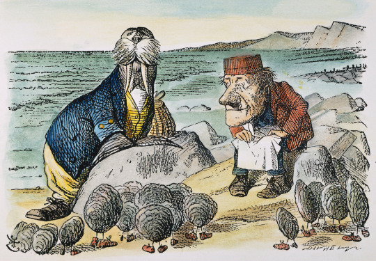
“O Oysters, come and walk with us!” The Walrus did beseech. “A pleasant walk, a pleasant talk, Along the briny beach: We cannot do with more than four, To give a hand to each.”

* * *

“The time has come,” the Walrus said, “To talk of many things: Of shoes–and ships–and sealing-wax– Of cabbages–and kings– And why the sea is boiling hot– And whether pigs have wings.”

-Lewis Carroll, The Walrus and the Carpenter

In this segment, probable numbers will be shown to grow out of a natural context inherently rather than through geometric second thought as transpired  in the history of Western thought  with imaginary numbers and complex plane.  To continue  with development of probable numbers it will be necessary to leave behind,  for the time being,  all preoccupation with imaginary numbers and complex plane.  It will also be necessary  to depart from our comfort zone of Cartesian spatial coordinate axioms and orientation.

Probable coordinates do not negate validity of Cartesian coordinates but they do relegate them to the status of a special case.  In the probable coordinate system the three-dimensional coordinate system of Descartes maps only one eighth of the totality. This means then, that the Cartesian two-dimensional coordinate plane furnishes just one quarter of the total number of  corresponding probable coordinate mappings  projected to a two-dimensional space.^[1]  It suggests also that  Cartesian localization  in 2-space or 3-space is just a small part of the whole story regarding actual spatial and temporal locality and their accompanying physical capacities, say for instance of momentum or mass, but actually encompassing a host of other competencies as well.

Although this might seem strange it is a good thing. Why is it a good thing?  First, because nature, as a self-sustaining reality, cannot favor any one coordinate scheme but must encompass all possible - if it is to realize any.  Second,  because both the Schrödinger equationandFeynman path integral approaches to quantum mechanics say it is so.^[2]  Third,  because Hilbert space demands it.  This may leave us disoriented and bewildered, but nature revels in this plan of probable planes. Who are we to argue?

So how do we accomplish this feat? Well, basically by reflections in all dimensions and directions. We extend the Cartesian vectors every way possible.  That would give us  a 3 x 3 grid or lattice  of coordinate systems (the original Cartesian system  and  eight new grid elements surrounding it),  but there are only four different types,  so we require only four of the nine to demonstrate. It is best not to show all nine in any case because to do so  would place our Cartesian system at direct center of this geometric probable universe and that would be misleading. Why? Because when we tile the two-dimensional universe to infinity in all directions,  there is no central coordinate system. Any one of the four could be considered at the center, so none actually is. Overall orientation is nondiscriminative.^[3]

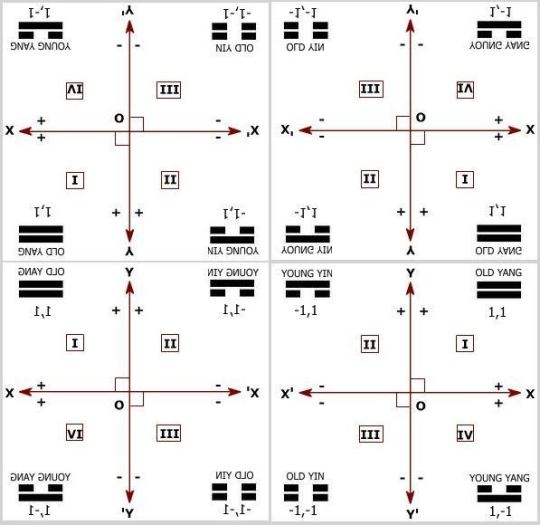
LOOKING GLASS CARTESIAN COORDINATE QUARTET

The image seen immediately above shows four  Looking House Cartesian coordinate systems, correlated within a mandalic plane. This mandalic plane is  one of six faces of a mandalic cube,  each of which  is constructed to a different plan but composed of similar building blocks, the four bigrams in various positions and orientations. A 2-dimensional geometric universe can be tiled with this image,  recursively repeating it in all directions throughout the two dimensions.^[4] It should not be very difficult for the reader to determine which of the four mandalic moieties references our particular conventional Cartesian geometric universe.^[5]

It remains only to be added here and now that potential dimensions, probable planes,  and  probable numbers  arise  immediately and directly from the remarks above. In some ways it’s a little like valence in chemical reactions.  We’ll likely take a look at that combinatory dynamic in context of mandalic geometry at some time down the road.  Next though we want to see how the addition of composite dimension impacts and modifies the basic geometry of the probable plane discussed here.^[6]

(to be continued)

Top image: The four quadrants of the Cartesian plane.  These are numbered in the counterclockwise direction by convention. Architectonically, two number lines are placed together, one going left-right and the other going up-down to provide context for the two-dimensional plane.  This image has been modified from one found here.

Notes

[1] To clarify further:  There are eight possible Cartesian-like orientation variants in mandalic space arranged around a single point at which they are all tangent to one another. If we consider just the planar aspects of mandalic space,  there are  four possible Cartesian-like orientation variants  which are organized about a central shared point in a manner similar to how quadrants are symmetrically arranged  about the Cartesian origin point (0,0) in ordinary 2D space. But here the center point determining symmetries is always one of the points showing greatest rather than least differentiation. That is to say it is formed by Cartesian vertices, ordered pairs having all 1s, no zeros.  That may have confused more than clarified, but it seemed important to say.  We will be expanding on these thoughts in posts to come. Don’t despair. For just now the important takeaway is that the mandalic coordinate system combines two very important elements that optimize it for quantum application:  it manages to be both probabilistic and convention-free  (in terms of spatial orientation,  which surely must relate to quantum states and numbers in some as yet undetermined manner.) At the same time, imaginary numbers and complex plane are neither.

[2] Even if physics doesn’t yet (circa 2016) realize this to be true.

[3] It is an easy enough matter to extrapolate this mentally to encompass the Cartesian three-dimensional coordinate system but somewhat difficult to demonstrate in two dimensions.  So we’ll persevere with a two-dimensional exposition for the time being. It only needs to be clarified here that the three-dimensional realization involves a 3 x 3 x 3 grid but requires just eight cubes to demonstrate because there are only eight different coordinate system types.

[4] I am speaking here in terms of ordinary dimensions but it should be understood that the reality is that the mandalic plane is a composite 4D/2D geometric structure, and the mandalic cube is a composite 6D/3D structure. The image seen here does not fully clarify that because it does not yet take into account composite dimension nor place the bigrams in holistic context within tetragrams and hexagrams.  All that is still to come.  Greater context will make clear how composite dimension works and why it makes eminent good sense for a self-organizing universe to invoke it. Hint: it has to do with quantum interference phenomena and is what makes all process possible.

ADDENDUM (12 APRIL, 2016)
The mandalic plane I am referring to here corresponds to the Cartesian 2-dimensional plane and is based on four extraordinary dimensions that are composited to the ordinary two dimensions, hence hybrid 4D/2D. It should be understood though that any number of extra dimensions could potentially be composited to two or three ordinary dimensions. The probable plane described in this post is not such a mandalic plane as no compositing of dimensions has yet been performed. What is illustrated here is an ordinary 2-dimensional plane that has undergone reflections in x- and y-dimensions of first and second order to form a noncomposited probable plane. The distinction is an important one.

[5] This is perhaps a good place to mention that the six  planar faces  of the mandalic cube fit together seamlessly in 3-space,  all mediated by the common shared central point, in Cartesian terms the origin at ordered triad (0.0.0) where eight hexagrams coexist in mandalic space. Moreover the six planes fit together mutually by means of a nuclear particle-and-force equivalent of the mortise and tenon joint but in six dimensions rather than two or three, and both positive and negative directions for each.

[6] It should also be avowed that tessellation of a geometric universe with a nondiscriminative, convention-free coordinate system need not exclude use of Cartesian coordinates entirely in all contextual usages.  Where useful they can still be applied in combination with mandalic coordinates since the two can be made commensurate,  irrespective of  specific Cartesian coordinate orientation locally operative. Whatever the Cartesian orientation might be it can always be overlaid with our conventional version of the same. More concretely, hexagram Lines can be annotated with an ordinal numerical subscript specifying Cartesian location in terms of our  local convention  should it prove necessary or desirable to do so for whatever reason.

On the other hand,  before prematurely throwing out the baby with the bath water, we might do well to ask ourselves whether these strange juxtapositions of coordinates might not in fact encode the long sought-after hidden variables that could transform quantum mechanics into a complete theory.  In mandalic coordinates of the reflexive nature described, these so-called hidden variables could be hiding in plain sight.  Were that to prove the case,  David Bohm andLouis de Broglie  would be  immediately and hugely vindicated  in advancing their  pilot-wave theory of quantum mechanics.  We could finally consign the Copenhagen Interpretation to the scrapheap where it belongs,  along with both imaginary numbers and the complex plane.

ADDENDUM (24 APRIL, 2016)
Since writing this I’ve learned that de Broglie disavowed Bohm’s pilot wave theory upon learning of it in 1952. Bohm had derived his interpretation of QM from de Broglie’s original interpretation but de Broglie himself subsequently converted to Niels Bohr’s prevailing Copenhagen interpretation.

© 2016 Martin Hauser

Please note:  The content and/or format of this post may not be in finalized form. Reblog as a TEXT post will contain this caveat alerting readers to refer to the current version in the source blog. A LINK post will itself do the same. :)

Scroll to bottom for links to Previous / Next pages (if existent).  This blog builds on what came before so the best way to follow it is chronologically. Tumblr doesn’t make that easy to do. Since the most recent page is reckoned as Page 1 the number of the actual Page 1 continually changes as new posts are added.  To determine the number currently needed to locate Page 1 go to the most recent post which is here. The current total number of pages in the blog will be found at the bottom. The true Page 1 can be reached by changing the web address mandalicgeometry.tumblr.com to mandalicgeometry.tumblr.com/page/x, exchanging my current page number for x and entering.  To find a different true page(p) subtract p from x+1 to get the number(n) to use. Place n in the URL instead of x (mandalicgeometry.tumblr.com/page/n) where
n = x + 1 - p. :)

-Page 311-

Beyond the Enlightenment Rationalists:
From imaginary to probable numbers - III

(continued from here)

My objection to the imaginary dimension is not that we cannot see it.  Our senses cannot identify probable dimensions either, at least not in the visually compelling manner they can the three Cartesian dimensions. The question here is not whether imaginary numbers are mathematically true. How could they not be? The cards were stacked in their favor. They were defined in such a manner, – consistently and based on axioms long accepted valid, – that they are necessarily mathematically true. There’s a word for that sort of thing. –The word is  tautological.– No,  the decisive question is whether imaginary numbers apply to the real world; whether they are scientifically true, and whether physicists can truly rely on them to give empirically verifiable results with maps that accurately reproduce mechanisms actually used in nature.^[1]

The geometric interpretation of imaginary numbers was established as a belief system using the Cartesian line extending from  -1,0,0  through the origin  0,0,0 to 1,0,0  as the sole real axis left standing in the complex plane. In 1843,  William Rowan Hamilton introduced two additional axes in a quaternion coordinate system.  The new jandk axes,  similar to the i axis, encode coordinates of imaginary dimensions.  So the complex plane has one real axis, one imaginary; the quaternion system, three imaginary axes, one real, to accomplish which though involved loss of commutative multiplication. The mandalic coordinate system has three real axes upon which are superimposed six probable axes. It is both fully commensurate with the Cartesian system of real numbers  and  fully commutative for all operations throughout all dimensions as well.^[2]

All of these coordinate systems have a central origin point which all other points use as a locus of reference to allow clarity and consistency in determination of location.  The  mandalic coordinate system  is unique in that this point of origin is not a  null point of emptiness as in all the other locative systems,  but  a point of effulgence.  In that location  where occur Descartes’ triple zero triad (0.0.0) and the complex plane’s real zero plus imaginary zero (ax=0,bi=0), we find eight related hexagrams, all having neutral charge density,  each of these consisting of  inverse trigrams  with corresponding Lines of opposite charge, canceling one another out. These eight hexagrams are the only hexagrams out of sixty-four total possessing both of these characteristics.^[3]

So let’s begin now to plot the points of the mandalic coordinate system with  the view  of comparing its  dimensions and points  with  those of the complex plane.^[4]  The eight  centrally located hexagrams  all refer to  and are commensurate with the Cartesian triad (0,0,0). In a sense they can be considered eight  alternative possible states  which can  exist in this locale at different times. These are hybrid forms of the four complementary pair of hexagrams found at antipodal vertices of the mandalic cube.  The eight vertex hexagrams are those with upper and lower trigrams identical. This can occur nowhere else in the mandalic cube because there are only eight trigrams.^[5]

From the origin multiple probability waves of dimension radiate out toward the  central points of the faces of the cube,  where these divergent force fields rendezvous and interact with reciprocal forces returning from the eight vertices at the periphery. converging toward the origin.  Each of these points at the six face centers  are  common intersections  of another eight particulate states or force fields analogous to the origin point except that four originate within this basic mandalic module and four without in an adjacent tangential module. Each of the six face centers then is host to four internal resident hexagrams which  share the point in some manner, time-sharing or other. The end result is the same regardless, probabilistic expression of  characteristic form and function.  There is a possibility that this distribution of points and vectors  could be or give rise to a geometric interpretation of the Schrödinger equation,  the fundamental equation of physics for describing quantum mechanical behavior. Okay, that’s clearly a wild claim, but in the event you were dozing off you should now be fully awake and paying attention.

The vectors connecting centers of opposite faces of an ordinary cube through the cube center or origin of the Cartesian coordinate system are at 180° to each other forming the three axes of the system corresponding to the number of dimensions.  The mandalic cube has 24 such axes, eight of which accompany each Cartesian axis thereby shaping a hybrid 6D/3D coordinate system. Each face center then hosts internally four hexagrams formed by  hybridization of trigrams  in  opposite vertices  of diagonals of that cube face,  taking one trigram  (upper or lower)  from one vertex and the other trigram (lower or upper) from the other vertex. This means that a face of the mandalic cube has eight diagonals, all intersecting at the face center, whereas a face of the ordinary cube has only two.^[6]

The circle in the center of this figure is intended to indicate that the two pairs of antipodal hexagrams at this central point of the cube face rotate through 90° four times consecutively to complete a 360° revolution. But I am describing the situation here in terms of revolution only to show an analogy to imaginary numbers.  The actual mechanisms involved can be better characterized as inversions (reflections through a point),  and the bottom line here is that for each diagonal of a square, the corresponding mandalic square has  a possibility of 4 diagonals;  for each diagonal of a cube,  the corresponding mandalic cube has a possibility of 8 diagonals. For computer science, such a multiplicity of possibilities offers a greater number of logic gates in the same computing space and the prospect of achieving quantum computing sooner than would be otherwise likely.^[7]

Similarly, the twelve edge centers of the ordinary cube host a single Cartesian point,  but the superposed mandalic cube hosts two hexagrams at the same point. These two hexagrams are always inverse hybrids of the two vertex hexagrams of the particular edge.  For example,  the edge with vertices  WIND over WIND  and  HEAVEN over HEAVEN  has as the two hybrid hexagrams  at the  center point  of the edge  WIND over HEAVEN  and HEAVEN over WIND. Since the two vertices of concern here connect with one another  via  the horizontal x-dimension,  the two hybrids  differ from the parents and one another only in Lines 1 and 4 which correspond to this dimension.  The other four Lines encode the y- amd z-dimensions, therefore remain unchanged during all transformations undergone in the case illustrated here.^[8]

This post began as a description of the structure of the mandalic coordinate system and how it differs from those of the complex plane and quaternions.  In the composition,  it became also  a passable introduction to the method of  composite dimension.  Additional references to the way composite dimension works  can be found scattered throughout this blog and Hexagramium Organum.  Basically the resulting construction can be thought of as a  tensegrity structure,  the integrity of which is maintained by opposing forces in equilibrium throughout, which operate continually and never fail,  a feat only nature is capable of.  We are though permitted to map the process  if we can manage to get past our obsession with  and addiction to the imaginary and complex numbers and quaternions.^[9]

In our next session we’ll flesh out probable dimension a bit more with some illustrative examples. And possibly try putting some lipstick on that PIG (Presumably Imaginary Garbage) to see if it helps any.

(continuedhere)

Image: A drawing of the first four dimensions. On the left is zero dimensions (a point) and on the right is four dimensions  (A tesseract).  There is an axis and labels on the right and which level of dimensions it is on the bottom. The arrows alongside the shapes indicate the direction of extrusion. By NerdBoy1392 (Own work) [CC BY-SA 3.0orGFDL],via Wikimedia Commons

Notes

[1] For more on this theme,  regarding quaternions,  see Footnote [1]  here. My own view is that imaginary numbers, complex plane and quaternions are artificial devices, invented by rational man, and not found in nature.  Though having limited practical use in  representation of rotations  in  ordinary space they have no legitimate application to quantum spaces,  nor do they have any substantive or requisite relation to square root, beyond their fortuitous origin in the Rationalists’ dissection and codification of square root historically, but that part of the saga was thoroughly misguided.   We wuz bamboozled.  Why persist in this folly? Look carefully without preconception and you’ll see this emperor’s finery is wanting. It is not imperative to use imaginary numbers to represent rotation in a plane. There are other, better ways to achieve the same. One would be to use sin and cos functions of trigonometry which periodically repeat every 360°.  (Read more about trigonometric functions here.)  Another approach would be to use polar coordinates.

[SOURCE]

A quaternion, on the other hand,  is a four-element vector composed of a single real element and three complex elements. It can be used to encode any rotation in a  3D coordinate system.  There are other ways to accomplish the same, but the quaternion approach offers some advantages over these.  For our purposes here what needs to be understood is that mandalic coordinates encode a hybrid 6D/3D discretized space. Quaternions are applicable only to continuous three-dimensional space.  Ultimately,  the two reside in different worlds and can’t be validly compared. The important point here is that each has its own appropriate domain of judicious application. Quaternions can be usefully and appropriately applied to rotations in ordinary three-dimensional space, but not to locations or changes of location in quantum space.  For description of such discrete spaces, mandalic coordinates are more appropriate, and their mechanism of action isn’t rotation but inversion (reflection through a point.) Only we’re not speaking here about inversion in Euclidean space, which is continuous, but in discrete space, a kind of quasi-Boolean space,  a higher-dimensional digital space  (grid or lattice space). In the case of an electron this would involve an instantaneous jump from one electron orbital to another.

[2] I think another laudatory feature of mandalic coordinates is the fact that they are based on a thought system that originated in human prehistory, the logic of the primal I Ching. The earliest strata of this monumental work are actually a compendium of combinatorics and a treatise on transformations,  unrivaled until modern times, one of the greatest intellectual achievements of humankind of any Age.  Yet its true significance is overlooked by most scholars, sinologists among them.  One of the very few intellectuals in the West who knew its true worth and spoke openly to the fact, likely at no small risk to his professional standing, was Carl Jung, the great 20th century psychologist and philosopher.

It is of relevance to note here that all the coordinate systems mentioned are, significantly,  belief systems of a sort.  The mandalic coordinate system  goes beyond the others though,  in that it is based on a still more extensive thought system, as the primal I Ching encompasses an entire cultural worldview.  The question of which,  if any,  of these coordinate systems actually applies to the natural order is one for science, particularly physics and chemistry, to resolve.

Meanwhile, it should be noted that neither the complex plane nor quaternions refer to any dimensions beyond the ordinary three, at least not in the manner of their current common usage.  They are simply alternative ways of viewing and manipulating the two- and three-dimensions described by Euclid and Descartes. In this sense they are little different from  polar coordinatesortrigonometry  in what they are attempting to depict.  Yes, quaternions apply to three dimensions, while polar coordinates and trigonometry deal with only two.  But then there is the method of  Euler angles  which describes orientation of a rigid body in three dimensions and can substitute for quaternions in practical applications.

A mandalic coordinate system, on the other hand, uniquely introduces entirely new features in its composite potential dimensions and probable numbers which I think have not been encountered heretofore. These innovations do in fact bring with them  true extra dimensions beyond the customary three  and also the novel concept of dimensional amplitudes.  Of additional importance is the fact that the mandalic method relates not to rotation of rigid bodies,  but to interchangeability and holomalleability of parts  by means of inversions through all the dimensions encompassed, a feature likely to make it useful for explorations and descriptions of particle interactions of quantum mechanics.  Because the six extra dimensions of mandalic geometry may, in some manner, relate to the six extra dimensions of the 6-dimensional Calabi–Yau manifold, mandalic geometry might equally be of value in string theoryandsuperstring theory.

Itis possible to use mandalic coordinates to describe rotations of rigid bodies in three dimensions,  certainly,  as inversions can mimic rotations, but this is not their most appropriate usage. It is overkill of a sort. They are capable of so much more and this particular use is a degenerate one in the larger scheme of things.

[3] This can be likened to a quark/gluon soup.  It is a unique and very special state of affairs that occurs here. Physicists take note. Don’t let any small-minded pure mathematicians  dissuade you from the truth.  They will likely write all this off as “sacred geometry.” Which it is, of course, but also much more.  Hexagram superpositions  and  stepwise dimensional transitions  of the mandalic coordinate system could hold critical clues  to  quantum entanglement and quantum gravity. My apologies to those mathematicians able to see beyond the tip of their noses. I was not at all referring to you here.

[4] Hopefully also with dimensions and points of the quaternion coordinate system once I understand the concepts involved better than I do currently. It should meanwhile be underscored that full comprehension of quaternions is not required to be able to identify some of their more glaring inadequacies.

[5] In speaking of  "existing at the same locale at different times"  I need to remind the reader and myself as well that we are talking here about  particles or other subatomic entities that are moving at or near the speed of light,- - -so very fast indeed. If we possessed an instrument that allowed us direct observation of these events,  our biologic visual equipment  would not permit us to distinguish the various changes taking place. Remember that thirty frames a second of film produces  the illusion of motion.  Now consider what  thirty thousand frames  a second  of  repetitive action  would do.  I think it would produce  the illusion of continuity or standing still with no changes apparent to our antediluvian senses.

[6] Each antipodal pair has four different possible ways of traversing the face center.  Similarly,  the mandalic cube has  thirty-two diagonals  because there are eight alternative paths by which an antipodal pair might traverse the cube center. This just begins to hint at the tremendous number of  transformational paths  the mandalic cube is able to represent, and it also explains why I refer to dimensions involved as  potentialorprobable dimensions  and planes so formed as probable planes.  All of this is related to quantum field theory (QFT), but that is a topic of considerable complexity which we will reserve for another day.

[7] One advantageous way of looking at this is to see that the probabilistic nature of the mandalic coordinate system in a sense exchanges bits for qubits and super-qubits through creation of different levels of logic gates that I have referred to elsewhere as different amplitudes of dimension.

[8] Recall that the Lines of a hexagram are numbered 1 to 6, bottom to top. Lines 1 and 4 correspond to, and together encode, the Cartesian x-dimension. When both are yang (+),  application of the method of  composite dimension results in the Cartesian value  +1;  when both yin (-),  the Cartesian value  -1. When either Line 1 or Line 4 is yang (+) but not both (Boole’s exclusive OR) the result is one of two possible  zero formations  by destructive interference. Both of these correspond to (and either encodes) the single Cartesian zero (0). Similarly hexagram Lines 2 and 5 correspond to and encode the Cartesian y-dimension; Lines 3 ane 6, the Cartesian z-dimension. This outline includes all 9 dimensions of the hybrid  6D/3D coordinate system:  3 real dimensions and the 6 corresponding probable dimensions. No imaginary dimensions are used; no complex plane; no quaternions. And no rotations. This coordinate system is based entirely on inversion (reflection through a point)  and on constructive or destructive interference. Those are the two principal mechanisms of composite dimension.

[9] The process as mapped here is an ideal one.  In the real world errors do occur from time to time. Such errors are an essential and necessary aspect of evolutionary process. Without error, no change. And by implication, likely no continuity for long either, due to external damaging and incapacitating factors that a natural world devoid of error never learned to overcome.  Errors are the stepping stones of evolution, of both biological and physical varieties.

Beyond Descartes - Part 6

The Fiction Formerly Known As the Line

(continued from here)

Rereading the last post a moment ago I see I fell into the same old trap, namely describing a concept arising from an alternative worldview in terms of our Western worldview.  It is so astonishingly easy to do this. So it is important always to be on guard against this error of mind.

In saying that the Taoist number line is the basis of its coordinate system I was phrasing the subject in Western terminology,  which doesn’t just do an injustice to the truth of the matter,  it does violence to it,  in the process destroying the reality:  that within Taoism, the coordinate system is primary.  It precedes the line,  which follows from it.  What may be the most important difference between the Taoist apprehension of space and that of Descartes lies encoded within that single thought.

Descartes continues the fiction fomented in the Western mind by Euclid that  the point and the line  have independent reality. Taking that to be true,  Descartes constructs his coordinate system using  pointsandlines  as the elemental building blocks. But to be true to the content and spirit of Taoism, this fabrication must be surrendered.  For Taoism,  the coordinate system, which models space, or spacetime rather, is primary. Therefore to understand the fictional Taoist line we must begin there, in the holism and the complexity of its coordinate system where dimension, whatever it may be, reigns supreme.^[1]

And that means we can no longer disregard composite dimension, postponing discussion of it for a later time,  because it is the logical basis on which the I Ching is predicated. It is related to what we today know as combinatorics,Boolean algebra, and probability,  and is what gives rise to what I have called the plane of potentiality. It is the very pith of mandalic geometry, what makes it a representation of mandalic spacetime.^[2]

(continuedhere)

Notes

[1] In my mind, dimension is a category of physical energetic description before it is a category of geometrical description.  When particle physicists speak about “quantum numbers” I think they are actually, whether intended or not, referring to dimensions. If this is true, then our geometries should be constructed to reflect that primordial reality, not arbitrarily as we choose.

[2] In speaking of logic and the I Ching in the same breath I am using the term in its broadest sense as any formal system in which are defined axioms and rules of inference. In reference to the I Ching,  the logic involved is far removed from the rationalism bequeathed to Descartes by his times.  It is a pre-rationalist logic that prevailed in human history for a very long time before the eventual splitting off of the irrational from the rational.  This means also that the I Ching is among other things a viable instrument to access strata of human minds long dormant in historical times,  other than possibly,  at times,  in poetry and art and the work of those select scientists who make extensive use of intuition in the development of their theories.

Note to self:  Two contrasting systems of thought based on very different worldviews can never be adequately explained in terms of one another. At times though, for lack of anything better, we necessarily fall back on just such a strategy, however limited, and make the best of it we can.

© 2015 Martin Hauser

Please note:  The content and/or format of this post may not be in finalized form. Reblog as a TEXT post will contain this caveat alerting readers to refer to the current version in the source blog. A LINK post will itself do the same. :)

Scroll to bottom for links to Previous / Next pages (if existent).  This blog builds on what came before so the best way to follow it is chronologically. Tumblr doesn’t make that easy to do. Since the most recent page is reckoned as Page 1 the number of the actual Page 1 continually changes as new posts are added.  To determine the number currently needed to locate Page 1 go to the most recent post which is here. The current total number of pages in the blog will be found at the bottom. The true Page 1 can be reached by changing the web address mandalicgeometry.tumblr.com to mandalicgeometry.tumblr.com/page/x, exchanging my current page number for x and entering.  To find a different true page(p) subtract p from x+1 to get the number(n) to use. Place n in the URL instead of x (mandalicgeometry.tumblr.com/page/n) where
n = x + 1 - p. :)

-Page 282-

18.09.2019

hope everyone is having a lovely september ☕️

If you were a martingale, would you rather be a submartingale or a supermartingale?

No you can’t have p=q.

the-real-numbers:

mathgirl:

mathgirl:

Do you think, in the whole history of Minecraft, any two players have ever generated the same random seed and therefore started on the exact same world, just by chance?

I thought about this while watching random seed minecraft speedrun attempts, where runners will constantly generate new worlds and try to beat the game in a random new world each time. I’m going to investigate the probability, but it would involve a guess about just how many new worlds are randomly generated every day. Any ideas?

Sources are telling me that Minecraft has sold over 200 million copies. Some of those copies are owned by avid players who have generated hundreds or even thousands of new worlds during their lives. I’d imagine many more copies are owned by people who haven’t spent much time on it, and only created one or two new worlds, or even zero.

I’m gonna take a wild guess and say the average number of new worlds generated in any given Minecraft game is 10. With 200 million copies sold, this estimates that 2 billion worlds have been generated and played in.

TheMinecraft fan wiki tells me that in Java edition, there are 2^48 possible seeds that can generate meaningful, unique worlds. (To keep things simple, I’m ignoring differences between bedrock and java editions here.)

The question I’m asking is: what are the chances that two players have ever generated the exact same seed by chance? Or inversely: what are the chances that every seed generated so far has been unique? This is equivalent to the Birthday Paradox, which I’d love to discuss in detail, but I’ll try to keep it brief.

The birthday paradox asks the question: in a room full of people, what are the chances that two people share the same birthday? You can think of a person’s birthday like some random value from 1 to 365 that is assigned to them (excluding February 29 for the sake of simplicity; sorry leap year babies). Any two people have a pretty low chance of having the same birthday, but this problem is called a paradox because the answer isn’t intuitive, and the odds are higher than you’d expect. In a room of 23 people, there’s a more than 50% chance that two individuals share a birthday.

Rather than going over the math here, I’ll let you check it out on wikipedia, but it basically boils down to this: add people to the group one-by-one, and check the likelihood of everyone in the group having a different birthday. The first person is alone, and therefore has a 100% chance of having a unique birthday. Add a second person. In order for their birthday to be unique, it has to fall on one of the 364 days that aren’t the first person’s birthday, giving them a very high 364/365 chance of having a unique birthday. The pool of possible unique birthdays shrinks again for the third person, but they still have a 363/365 chance of being unique. And so on.

I won’t get into the pigeonhole principle, fascinating as it is, since it isn’t relevant to our Minecraft problem. Hopefully you can see that if you replace the days of the year with possible random seeds, and replace people in a room with randomly generated seeds, it’s the same exact question.

Wikipedia helpfully shows us how to calculate the probability that a group of n people all have unique birthdays, and gives us this formula:

Just replace 365 with our total potential number of seeds (2^48) and interpret n as the number of randomly generated worlds, and we’re well on the way to finding the chance that every generated world has been unique.

Er… the only problem is, these are quite big numbers to be calculating factorials and binomial coefficients for. I’m kind of scared to ask a machine to do that for me. Luckily, Wolfram Alpha has a built in birthday paradox calculator, but… it’s not quite up to the task either.

Um… help?

(This can be done with some kind of approximation, and I’ll try to tackle it later if nobody else gives it a shot)

(not to steal your thunder, but this looks like a fun computation. I do want to see if you get the same thing, I may have errors.)

You can use Stirling’s approximation (like you alluded to), and if you substitute 2^48 with a variable (here it’s alpha) it’s easy to simplify. I think you get this:

Note that the final formula in the circle is still an approximation but boy is it nice. And for numbers like 2^48 it should be pretty accurate.

So it seems we’re all getting answers that basically round to zero. Your approximation is mostly dominated by the 1/e^n term, which is very small for n as large as 2 billion. @galois-groupie​ attempted an approximation as well, which resulted in another negligible result. And I opted to try this Taylor approximation that wikipedia provided for the generalized birthday problem:

(note that this is the probability of getting two same birthdays, not the probability of all unique birthdays, so it’s the opposite of the result you guys found. Plugging in 2^48 for d and 2 billion for n gives a result that rounds to 1.)

So what does this mean for Minecraft? I think it’s safe to say that the chance of every randomly generated seed being unique is negligibly small, meaning it’s certain that two people somewhere have rolled the same seed. In fact, there are probably lots of seed soulmates out there. If you believe, then there’s a chance your favorite speedrunner may have stumbled across your own world seed while they were going for the world record.

I think the reason the result is so clear hearkens back to the birthday problem itself. Out of 365 possible birthdays you can have, the chance of two people sharing a birthday ramps up really fast for every person you introduce to the group.

This makes sense if you think about the number of pairs of people in a group, since that’s what you’re really checking when looking for a match. For every person you add, the web of pairs grows more complex. In the case of Minecraft, the number of pairs you can draw between 2 billion worlds is absolutely enormous. I just guessed those numbers, but I’m sure you’d get a similar result no matter what reasonable estimate you make.

This was a fun exercise! Thanks for the help. And good luck finding your Minecraft soulmate.

mathgirl:

Do you think, in the whole history of Minecraft, any two players have ever generated the same random seed and therefore started on the exact same world, just by chance?

I thought about this while watching random seed minecraft speedrun attempts, where runners will constantly generate new worlds and try to beat the game in a random new world each time. I’m going to investigate the probability, but it would involve a guess about just how many new worlds are randomly generated every day. Any ideas?

Sources are telling me that Minecraft has sold over 200 million copies. Some of those copies are owned by avid players who have generated hundreds or even thousands of new worlds during their lives. I’d imagine many more copies are owned by people who haven’t spent much time on it, and only created one or two new worlds, or even zero.

I’m gonna take a wild guess and say the average number of new worlds generated in any given Minecraft game is 10. With 200 million copies sold, this estimates that 2 billion worlds have been generated and played in.

TheMinecraft fan wiki tells me that in Java edition, there are 2^48 possible seeds that can generate meaningful, unique worlds. (To keep things simple, I’m ignoring differences between bedrock and java editions here.)

The question I’m asking is: what are the chances that two players have ever generated the exact same seed by chance? Or inversely: what are the chances that every seed generated so far has been unique? This is equivalent to the Birthday Paradox, which I’d love to discuss in detail, but I’ll try to keep it brief.

The birthday paradox asks the question: in a room full of people, what are the chances that two people share the same birthday? You can think of a person’s birthday like some random value from 1 to 365 that is assigned to them (excluding February 29 for the sake of simplicity; sorry leap year babies). Any two people have a pretty low chance of having the same birthday, but this problem is called a paradox because the answer isn’t intuitive, and the odds are higher than you’d expect. In a room of 23 people, there’s a more than 50% chance that two individuals share a birthday.

Rather than going over the math here, I’ll let you check it out on wikipedia, but it basically boils down to this: add people to the group one-by-one, and check the likelihood of everyone in the group having a different birthday. The first person is alone, and therefore has a 100% chance of having a unique birthday. Add a second person. In order for their birthday to be unique, it has to fall on one of the 364 days that aren’t the first person’s birthday, giving them a very high 364/365 chance of having a unique birthday. The pool of possible unique birthdays shrinks again for the third person, but they still have a 363/365 chance of being unique. And so on.

I won’t get into the pigeonhole principle, fascinating as it is, since it isn’t relevant to our Minecraft problem. Hopefully you can see that if you replace the days of the year with possible random seeds, and replace people in a room with randomly generated seeds, it’s the same exact question.

Wikipedia helpfully shows us how to calculate the probability that a group of n people all have unique birthdays, and gives us this formula:

Just replace 365 with our total potential number of seeds (2^48) and interpret n as the number of randomly generated worlds, and we’re well on the way to finding the chance that every generated world has been unique.

Er… the only problem is, these are quite big numbers to be calculating factorials and binomial coefficients for. I’m kind of scared to ask a machine to do that for me. Luckily, Wolfram Alpha has a built in birthday paradox calculator, but… it’s not quite up to the task either.

Um… help?

(This can be done with some kind of approximation, and I’ll try to tackle it later if nobody else gives it a shot)

Do you think, in the whole history of Minecraft, any two players have ever generated the same random seed and therefore started on the exact same world, just by chance?

I thought about this while watching random seed minecraft speedrun attempts, where runners will constantly generate new worlds and try to beat the game in a random new world each time. I’m going to investigate the probability, but it would involve a guess about just how many new worlds are randomly generated every day. Any ideas?

1/8192. This might be a fraction you’ve heard quoted as the probability of encountering a shiny pokemon. Perhaps you heard 1/4096 if you’re playing a newer game, or an even better probability if you use some special techniques. But this chance turns out to be a downright miniscule, something that’s hard to wrap our heads around. How do you account for something that’s one in a thousand or more?

These odds are meant to be so rare that you can’t predict it happening. You may go a long time without seeing a shiny pokemon, but if you play long enough, you’re bound to encounter one as a pleasant surprise. Or if you’re a dedicated player, you may seek to increase your odds and purposefully get a shiny pokemon. In that case, how long can you expect your shiny hunt to last? How many hundreds of eggs will you need to hatch? How long can you go on until you decide you just have rotten luck? Join me, and we’ll take a delve into the realm of probability to answer some of these questions.

Let’s cut right to the heart of the matter: you’re a shiny hunter, and you’re looking to maximize your chances of encountering a shiny pokemon. There are plenty of places you can look up how to do this, so I’ll just state the results. I’ll assume you’ve filled the pokedex and earned your shiny charm. If you use the Masuda method of hatching eggs, each egg has a 1/512 chance of hatching shiny. If you have battled at least 500 of a particular wild pokemon, your chance of encountering its shiny form in the wild is the same, 1/512. These are the best odds you can get, perhaps barring some clever tricks with raid dens which I won’t cover here.

So you’ve got everything ready for your shiny hunt, and now you ask yourself the all-important question: how long is this going to take? Will I need to hatch 300 eggs? 600? A thousand? Probability is an area where our human intuition tends to fail, so this is where some calculations might help us understand the situation better.

The Math

We need to start by asking the right question. “How many eggs will I hatch before finding a shiny?” is a little too vague, because the answer could be anything. It’s a random process, and while the chance is slim, you could very well hatch a shiny on your first egg just as well as your 300th or 1000th. “If I hatch 300 eggs, what is the chance that one of them will be shiny?” is much better, because it gives us a concrete answer to look for: did I hatch a shiny, or not? What is the chance of each outcome? And we could ask that for any number of eggs: is there a significant chance of finding a shiny in a single box of 30 eggs? If my hunt goes on for 1000 eggs, what is my chance of finding success by then?

Stated as generally as possible, our question looks something like this:

For an event with probability P, what is the chance it will occur at least once in X number of trials?

Every time you hatch an egg or start a wild encounter, you can imagine drawing a number out of a hat with 512 numbered slips of paper in it, hoping that you’ll get the exact number you’re looking for. Each draw is independent: after you’ve drawn your slip of paper, you have to return it to the hat and shuffle them again, leaving each trial exactly the same. In the realm of probability, we call this kind of situation “drawing with replacement.” This means if you’ve hatched 1000 eggs already, your chance that the next one will be shiny is exactly the same as when you started.

Here’s the problem: I’m not much of a statistician. I don’t know the equations that govern these kinds of problems, so right away I can’t come up with an easy way to calculate the chance of hatching at least 1 shiny in 300 eggs or so. However, even without much knowledge of probability or statistics, a bit of clever thinking can get us what we’re looking for.

When it comes to questions of probability, I often find it’s easier to answer the opposite question. Above, we asked the probability of a rare event happening after a bunch of tries. What if, instead, we find the chance that it will neverhappen?

For an event with probability P, what is the chance it will not occur at all in X number of trials?

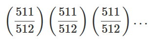
This is a question we can answer. If each egg has a 1/512 chance of hatching a shiny, then the remaining chance, 511/512, must be the chance of hatching a regular, non-shiny pokemon. That much is obvious; it’s a very high probability. If we hatch a bunch of eggs in a row, we can calculate the chance that they’ll all have the same non-shiny outcome by simply multiplying their independent probabilities together:

Notice that the fraction 511/512 is very close to 1, or a 100% probability, but not quite. It comes out to about 99.8%. This may seem insignificant, but the more of them we multiply together, the more the outcome will gradually decrease. It makes sense if you think about it: if you keep hatching eggs and getting regular non-shiny pokemon, there’s a good chance your streak will eventually be broken by a shiny pokemon (the outcome we ultimately want!).

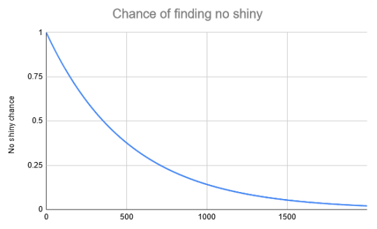
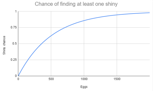
This chart shows what happens if you simply keep multiplying those probabilities together. If each one represents an egg hatched, then you can see once we hatch 1000 eggs or more, there’s a pretty slim chance that every single one will not be shiny, and that chance continues to approach zero.

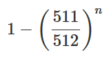
We’re very close to answering our original question. We’ve found the chance of hatching not a single shiny in a certain number of eggs. Now all we have to do is consider the other piece of the probability pie: if you failed in your attempt to hatch all regular pokemon, then it stands to reason you must have hatched at least one shiny. If the entire pie has a total of 1, or 100%, then we simply subtract off the probabilities we found to get the other situation:

Note that the exponent n refers to the number of eggs we hatch, and therefore the number of times to multiply our number 511/512 together. We’ve come to our answer in a roundabout way: this equation essentially says, what is the chance you will notfindno shinies in a batch of neggs?

This chart is encouraging. It shows us that within 300 eggs, we have about a 44% chance you’ll find your shiny by then. That’s pretty good! Some people I know have done shiny hunts that lasted about 300 eggs, so it matches real world experience. I got lucky enough to hatch a shiny pokemon in 85 eggs, and there’s about a 15% chance of that happening. Not exactly astronomical, but still lucky.

If you didn’t happen to find your shiny within the first couple hundred tries, don’t fret quite yet: you have an 86% chance of finding it within the first 1000. If you haven’t found it by then… well, you may have rotten luck, but keep trying. Your chances are still the same no matter what!

Here’s my favorite tidbit to come out of this calculation: when shiny hunting, I typically hatch eggs by the box, release them all when I fill up a box, and start again. For every batch of 30 randomly generated pokemon, there’s about a 5.7% chance at least one will be shiny. That’s a little better than 1/20, which gives me a useful way of visualizing my chances. Every time I start a new box, I can imagine rolling a 20-sided die and hoping for a 20.

My current shiny hunt has lasted up to 31 boxes, or 930 eggs without success. If you’re an intrepid shiny hunter like me, don’t give up– keep filling boxes, and eventually you’ll get your critical roll!

Final note: a lot of players can’t be bothered to fill the pokedex and acquire the shiny charm, so your shiny hunting odds may be different from mine. I encourage you to read over my calculations, plug in your own probabilities, and calculate some interesting values for yourself!

Death is a very little thing

Enough life and money has been spent on this sterile quest. The pole has already been discovered. What is the use of another expedition? Winston Churchill, then 1st Lord of the Admiralty, 23rd January, 1914 Dear Mr Winston Churchill, Do please look favourably … I am trying to do good and serious work … Death is a very little thing, and Knowledge very great … And really Regent Street holds out…

View On WordPress

This talk was given by Elizabeth Kelley at our student combinatorics seminar. She cited Godbole, Kurtz, Pralat, and Zhang as collaborators. One of these (Pralat, I think) was originally an editor, but then made substantial contributions to the project. This post is intended to be elementary.

[ Personal note: This is the last talk post I will be writing for OTAM. It seems fitting, since Elizabeth and I went to the same undergrad; I have actually known her for almost as long as I have been doing mathematics. ]

——

Acquisitions Incorporated

This is a graph theory talk, but, refreshingly, it did not begin with “Agraph is a pair of vertices andedges such that…”

It did begin with this: Let $G$ be a graph with a vertex-weighting (i.e. an assignment of nonnegative reals to each vertex). An acquisition move is a “complete transfer of weight” from a low-weight vertex to an adjacent higher-weight vertex. In other words, if the weights before the move are $w\leq x$, then the weights after the move are $0\leq w+x$ (respectively).

[ For the sake of not cluttering up the definitions with trivialities, we will say that both of the weights involved in an acquisition move must be strictly positive— that is: not zero. ]

From this, a bunch of definitions follow in quick succession. 

• A sequence of acquisition moves is called an acquisition protocol if it is maximal, i.e. after performing all of the moves, no further move is possible.
• The set of nonzero-weight vertices after performing an acquisition protocol is called a residual set.
• Finally, the acquisition number of $G$ is the minimum size of any residual set. We write it as $a(G)$.

This explains half of the title. The other half of the title, is perhaps a bit more self-explanatory. A lot is known about acquisition numbers when, say, all vertices are given weight $1$. Less is known in other contexts, but the goal of this paper is to ask what we “should” expect for paths. More precisely: if we give the vertices random weights, what is the expected acquisition number?

——

Fekete’s Lemma

A sequence of real numbers $(x_n)$ is called subadditive if it does what the name suggests: for all $n$ and $m$

$$ x_{n+m} \leq x_n + x_m.$$

This is a pretty general construction, and tons of sequences do this: certainly any decreasing sequence will, and also most reasonable sequences that grow slower than linear ($\log(n)$ works, for instance). Usually, when the situation is so general, it is hard to say anything at all about them, but in this case things are different:

Lemma (Fekete). Given any subadditive sequence $(x_n)$, the limit of $x_n/n$ exists, and moreover

$$ \lim_{n\to\infty} \frac{x_n}{n} = \text{inf}_n \frac{x_n}{n}. $$

(This lemma has one of my favorite proofs, which is essentially the same as the one given in this NOTSB post; just reverse all the inequalities and repeat the argument with liminf/limsup replaced by lim/inf.)

This means that whenever you have a subadditive sequence, it makes sense to ask about its growth rate, which is just the limit that Fekete guarantees exists. Less formally, it is the number $c$ such that $x_n \approx cn$ as $n$ gets large. (Perhaps in this formulation is the existence statement so striking: why should there be such a number at all? But Fekete states that there is.)

As it happens, it is pretty easy to prove that $a(P_n)$, where the path $P_n$ on $n$ vertices has been weighted with all 1s, forms a subadditive sequence.

This proof doesn’t use much about the weightings at all: it requires only that they are “consistent” in some technical sense. The punchline for our purposes is that $a(P_n)$ continues to form a subadditive sequence when the paths are weighted by independent identically distributed random variables.

——

Numbers, Please!

In the paper, Kelley considered the case when the vertex weights were distributed as a Poisson distribution. This is a thing whose details aren’t too important, but if you’re familiar with it you may be wondering why this instead of anything else? The answer is because when you know the answer for the Poisson model, you also know it in a more physically reasonable model: you start with a fixed amount of weight and you distribute it randomly to the vertices.

[ The process by which you use Poisson to understand the latter model is called “dePoissonization”, which makes me smile: to me it brings to mind images of someone hunched over their counter trying to scrub the fish smell out of it. ]

But enough justification: what’s the answer? Well, we don’t actually know the number on the nose, but here’s a good first step:

Theorem (Godbole–Kelley–Kurtz–Pralat–Zhang). Let the vertices of $P_n$ be weighted by Poisson random variables of mean $1$. Then $0.242n \leq \Bbb E[a(P_n)] \leq 0.375n$.

The proof of this theorem is mostly number-crunching, except for one crucial insight for each inequality: This step is easier to prove for the lower bound: after we have assigned numbers for the random variables, check which functions have been given the weight zero and look at the “islands” between them. Acquisition moves cannot make these islands interact, and so we can deal with them separately, so $\Bbb E[a(P_n)]$ splits up into a sum of smaller expectations based on the size of the islands. In a strong sense “most” of the islands will be small, and so you get a pretty good approximation just by calculating the first couple terms.

To get an upper bound, you need to think of strategies which will work no matter low long the path is and what variables are used. The most naïve strategy is to just pair off vertices of the path and send the smaller one in the pair to the larger one. This may or may not be an acquisition protocol, but you will always cut the residual set size (roughly) in half. Following even this naïve strategy is good enough to give the 0.375.

Both of these steps are fairly conceptually straightforward, but it becomes very difficult to calculate all the possibilities as you get further into the sum; in other words, it’s a perfect problem for looking to computer assistance. This allows us to get theoretical bounds $0.29523n \leq \Bbb E[a(P_n)] \leq 0.29576n$; and of course it would not be hard to get better results by computing more terms, but at some point it’s wiser to start looking for sharper theoretical tools rather than just trying to throw more computing power toward increasingly minuscule improvements.

Blaise Pascal

‘We know the truth, not only by the reason, but also by the heart.’

French mathematician and philosopher Blaise Pascal was born on this day in 1623. Educated by his father, Pascal showed an impressive grasp of mathematics from a young age, and went on to become a pioneer in the fields of game theory and probability. At the age of eighteen, in an effort to support his father with extensive tax calculations, he also invented and constructed one of the first mechanical calculators.

After an intense religious experience, Pascal’s commitment to Catholicism was renewed and he shifted his focus to religious, spiritual and philosophical writings. His most influential works are 'Lettres provinciales’ and 'Pensées’, the latter containing perhaps one of his most well-known ideas, Pascal’s Wager, which argues for a belief in God.

This small porcelain sculpture of Blaise Pascal was made in Sèvres Porcelain Factory c. 1784.